From IMF’s COFER:
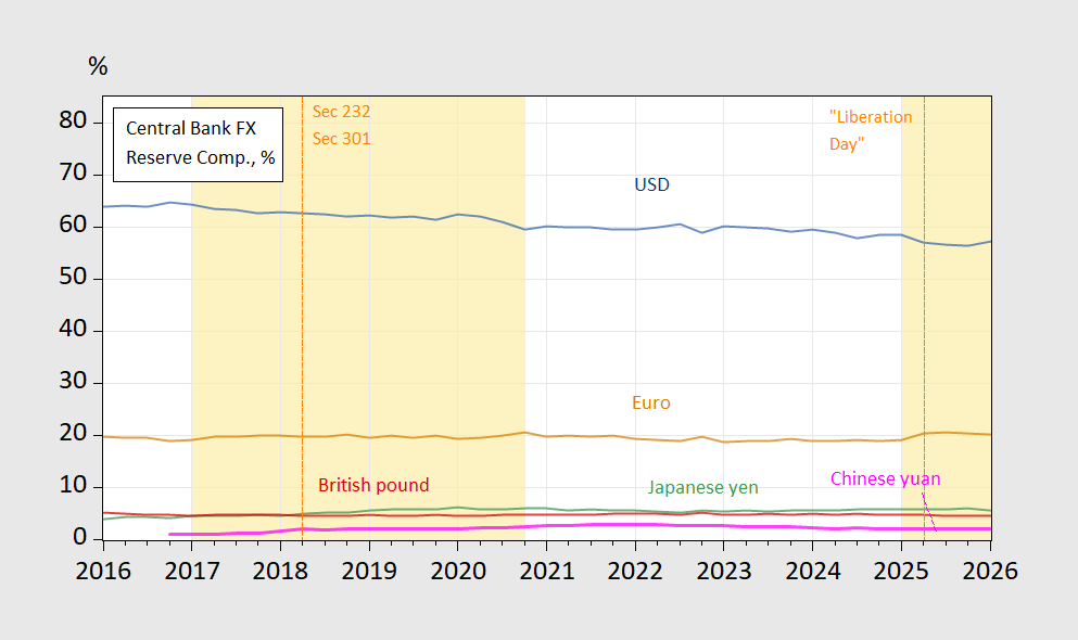
Figure 1: Share of total foreign exchange reserves for US dollar (blue), euro (brown), British pound (red), Japanese yen (green), Chinese yuan (pink), all in %. Orange shading denotes Trump Administrations. Source: IMF COFER (vers. June 30, 2026) and author’s calculations.
There’s a slight uptick in 2026Q1, in the wake of the war. Here’s a detail to make the change clearer.
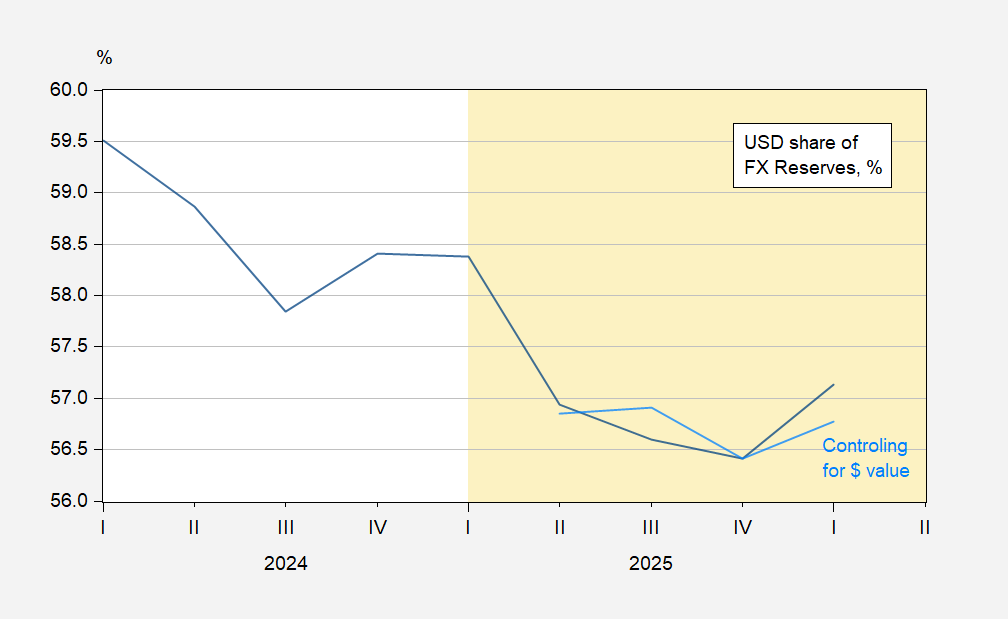
Figure 1: US dollar share of foreign exchange reserves (bold blue), share of foreign exchange reserves controlling for fx valuation effects at 2025Q4 rates (light blue). Controls for valuation using EUR, GBP, JPY echange rates. Source: IMF COFER (vers. June 30, 2026), FRED, and author’s calculations.
The uptick (from 56.4% to 57.1%) could arise from either flight to dollars, or valuation effects — i.e., the strengthening of the dollar. Controlling for valuation effects by using accounting for exchange rate changes against the dollar, the increase is less marked (to 56.8%).
OMFIF’s 2026 Public Investor Report notes:
…reserve managers remain cautious. While 56% of respondents intend to increase diversification, 54% plan to expand the size of their reserves.
So, once the war is resolved, one might expect a return to trend decline in dollar holdings, should the survey be accurate.
The Report also notes that gold is still being acquired as part of the the diversification drive; this showed up in the previous post on reserve holdings, but complete Q1 gold holdings are not yet available.
Total FX reserves in level are now re-attaining previous peaks, while total reserves (including gold have clearly exceeded prior peak.
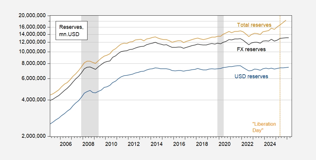
Figure 3: Reserves in USD (blue), foreign exchange reserves (black), foreign exchange plus gold reserves (brown), all in million USD, end-of-period, on log scale. NBER defined peak-to-trough recession dates shaded gray. Source: IMF COFER, Gold Council, NBER, and author’s calculations.
]]>