I made some comments on Sunday about a recent critique by Thomas Herndon, Michael Ash, and Robert Pollin of an influential 2010 paper by Carmen Reinhart and Kenneth Rogoff. Yesterday Econbrowser hosted a
reply from Pollin and Ash to my remarks. Here I would like to add a few further thoughts on this discussion.
Pollin and Ash first produce a graph that supports the statement I made that “At the moment, the interest rate on U.S. government debt is extremely low, so that despite our high debt load, the government’s net interest cost is currently quite reasonable.” However, they dismiss the possibility that interest rates may rise from their current low levels as merely the projections of “deficit hawks,” stating that
this pattern of low interest payments will almost certainly continue at least until the Fed alters its current monetary policy stance. Chair Bernanke has stated repeatedly that the Fed will continue with its current policy course at least until unemployment falls below 6.5 percent.
Pollin and Ash apparently did not follow the link I provided in support of my claim that many objective forecasters expect interest rates to rise. That link points to the discussion of long-term interest rates given by Ben Bernanke on March 1, in which the Fed chairman noted that predictions of rising interest rates have been made by (1) Blue Chip consensus forecast, (2) Survey of Professional Forecasters, (3) Congressional Budget Office, and (4) the Fed’s own interest rate model.
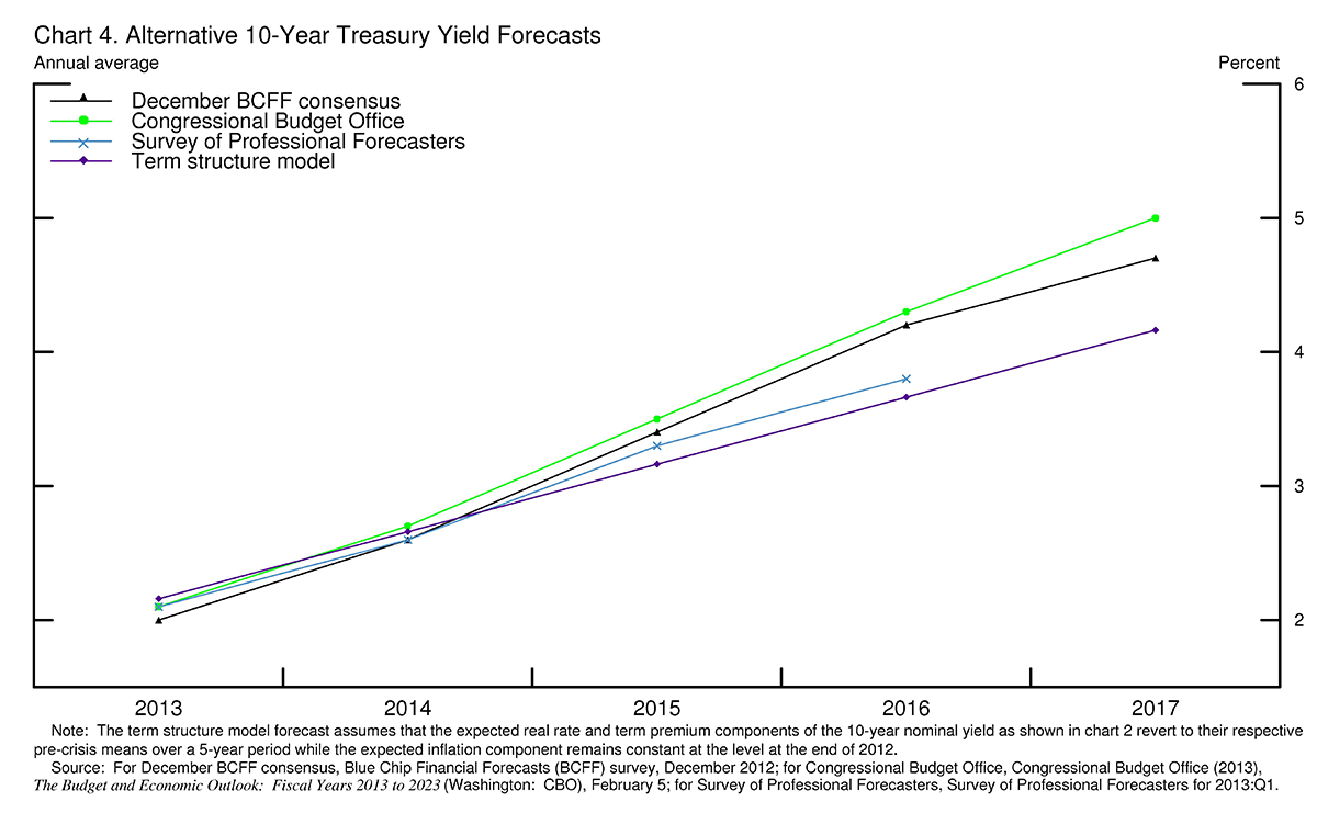 |
It is true that all four of these forecasts could be wrong– interest rates in 4 years could easily be higher or lower than those portrayed in the figure above. But if for example they follow the trajectory indicated by the green line, which is the baseline scenario recently constructed by the Congressional Budget Office, then net interest cost will be as big as the entire nondefense discretionary budget by 2018 and the entire defense budget by 2019.
Pollin and Ash then repeat the arguments in their paper about the desirability of treating all country-years equally without responding to the particular critique of their argument that I originally provided. The issue I raised has nothing to do with serial correlation. The issue instead is whether the expected GDP growth rate should be regarded as if it is the same number across different countries. A well-known econometric method for dealing with this is referred to as “country fixed effects.” In this method, one uses the average for the Greek observations as an estimate of the Greek growth rate and the average of the U.S. observations as an estimate of the U.S. growth rate. This is a widely used procedure. By contrast, the weighting proposed by Herndon, Ash, and Pollin assumes that the expected growth rate is the same across different countries, an approach that is less widely chosen for panel data sets and in my opinion less to be recommended. Given that the ultimate goal in this case is to infer an average effect across different countries, I personally feel that a random-effects approach would be superior to fixed-effects estimation, particularly given the unbalanced nature of the panel (that is, given the fact that we have many more observations on the 90% debt state for some countries than for others). As I noted in my original piece, this would yield an estimate that would be in between those or RR and HAP. But to suggest that there is some deep flaw in the method used by RR or obvious advantage to the alternative favored by HAP is in my opinion quite unjustified.
Finally, Pollin and Ash repeat the claim that the HAP estimates are substantially different from those in RR. Again, in doing so they have failed to respond to my original point, which was summarized in the table found here. To repeat, in Reinhart and Rogoff’s original (2010) paper there were separate analyses of three different data sets, and each data set was summarized using two different methods, the first based on means and the second based on medians. HAP had quarrels with only one of these three datasets (the postwar panel of advanced economies) and only one of the two methods (the sample means). F.F. Wiley has a helpful graph comparing the original RR summary of the postwar advanced data set using the median (blue in the graph below) with HAP’s summary of that same data set using HAP’s preferred reweighted means (in red).
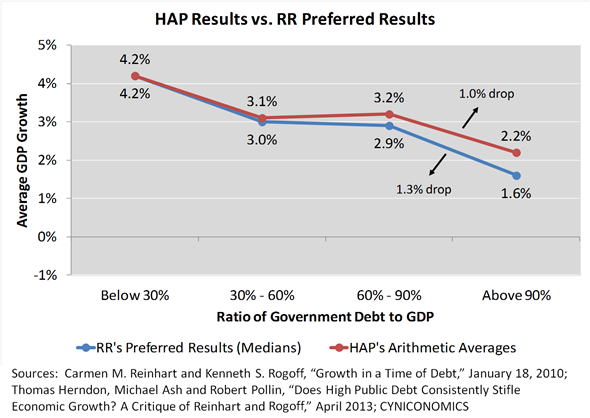 |
And for those Econbrowser readers who have been trying to point to this 2011 commentary by Reinhart and Rogoff as evidence of some claims that the HAP reanalysis somehow overturns, please note that the numbers Reinhart and Rogoff bring up in that article refer to the sample medians (blue lines) in the graph above.
A lot of us have “prediction of high interest rate” fatigue. A “good” prediction now faces the “chicken little” problem.
Even if you believe that there is a clear relationship (and the causality doesn’t go the other way round), don’t you require more than linear effects to justify modifying your behaviour given the debt level?
If an increase in debt causes a linear loss in growth, there should be no change in behaviour between 0% debt and 100% debt, since an increase in debt will cause the same loss irrespective of the starting point. It depends on what you achieve with whatever you buy with the resources you get from the debt.
Unless you argue that a country should never use debt, I don’t see how a linear relationship would change your decision.
Doesn’t it disturb you that there seems to be the same loss between 0-30 and 30-60 and 60-90 and 90-120? Frankly I don’t really understand how you can look at the massive effect relatively small changes in debt level can cause and have any trust in the relationship at all. How can increasing debt from 15% to 45% (an historically low level) hurt growth some much? I think it’s against all intuition and makes me question the validity of the exercise…
It’s simply breathtaking. Riddled with freshman errors and framed by their public statements then scooped up and adopted by the Masters of the Universe simply because it was what they wanted to hear. Reinhart-Rogoff is indefensible.
Shouldn’t we be talking about causality instead of averaging? I still fail to understand the contribution of R&R. Your last figure here plots change in X vs Y/X. Are we supposed to be surprised by the negative correlation? It seems quite clear that these results are only interesting if there is causality from Y/X to change in X. If R&R do not claim causality, then what is the contribution of this paper? And why are we still talking about it?
Prof. Hamilton, I have two comments.
First, regarding net interest cost and interest rate projections, isn’t it true that the $ value of any existing government bonds will fall as the interest rate rises? Why would you assume that the government would not buy back the existing debt at discounted prices? For example, $100BB of debt issued with a 1.8% rate (near current rates) Could be repurchased for $50BB (or their abouts) if rates were to double. Yes, net interest expense wouldn’t change, but the overall debt level would fall. And isn’t the current argument concerned with the debt/GDP level versus the net interest expense/GDP level?
Second, I keep seeing RR’s defenders posit the same argument re: RR’s medians vs. HAP’s averages. This is an apples and oranges comparison and you know it. A more rational argument would be to compare means to means or medians to medians. HAP, compares means to means, where RR show negative growth. IF you want to compare medians, then please state so but let’s ask HAP to provide their median results so that we can argue from the same starting line.
Wait, I’ll ask them…Tom, Michael and Bob, would you please provide your median results in each Debt/GDP range so that we can compare them to RR’s medians?
By the way, there is a good reason to prefer mean over median Professor and you know it.
Seems like I learn much more by reading a few paragraphs here than by reading any number of MSM stories regarding this debate, pro or con. Thank you for the excellent summary.
For the government to buy back debt it would need to cut spending or increase taxes, greatly.
Sebastian,
Indeed, and evidence does suggest causality:
More importantly, there is no tipping point as their paper and public statements suggested. It is in fact, a fairly straight gentle trend line.
Aaron,
For the government to buy back debt, all that is required is for a clerk in the NY Fed to tap, tap, tap on a computer keyboard to credit the bondholder’s bank account.
No spending cuts or tax increases required.
The Fed has been doing this to the tune of $85 billion a month for some time.
California would have to cut spending or raise taxes or borrow from someone to pay back a bond, but Uncle Sam does not.
“It is true that all four of these forecasts could be wrong– interest rates in 4 years could easily be higher or lower than those portrayed in the figure above. But if for example they follow the trajectory indicated by the green line, which is the baseline scenario recently constructed by the Congressional Budget Office, then net interest cost will be as big as the entire non-defense discretionary budget by 2018 and the entire defense budget by 2019.”
Just based on their past track record I would say it’s almost guaranteed that the forecasts of the 10-year rate are far too high. For example in 2009 the CBO was forecasting that the 10-year rate would be 5.4%. In 2010 they were forecasting 4.5%. In 2011 they were forecasting 4.2%. In 2012 they were forecasting 2.5%. This year they are forecasting 2.1%.
So far this year the 10-year rate has closed in the range of 1.72-2.07 and has averaged 1.91%.
Furthermore the past history of countries which have spent extended periods of time at or near the zero lower bound with large output gaps (e.g. the Great Depression, the Lost Decade etc.) strongly suggest that the 10-year rate will remain low for a very long time.
The CBO is forecasting net interest will rise to 2.5% of GDP in 2018 and 2.7% of GDP in 2019. The fact that those figures are more than the forecasted non-defense descretionary budget and defense budget respectively tells us much more about how little we plan to spend on descretionary items than it does about how high net interest will be. Even at those levels net interest will still be substantially less than the 3.25% of GDP it was in 1991.
Moreover, since I seriously doubt 10-year rates will be the 5.2% that the CBO is forecasting, I seriously doubt net interest will be anywhere near that high.
Any corporate treasurer worth his paycheck would be loading up on long-term low cost debt is faced with the treasury yield curve. What is wrong with the past and cirrent Secretary of the Treasury?
http://www.colbertnation.com/the-colbert-report-videos/425748/april-23-2013/austerity-s-spreadsheet-error
Forgive me, but am I correct in understanding that everyone is in agreement here?
1) Pollen and Ash state “this pattern of low interest payments will almost certainly continue at least until the Fed alters its current monetary policy stance.” JDH shows forecasts that predict a gradual rise in forecast long-term rates over four years. This two positions are not inconsistent with one another.
2) JDH notes that RR’s weighing experiences by country is defensible and advocates the use of “country fixed effects.” Pollen and Ash take the position that “to be reliable as a guide on important public policy issues, their results need to be robust to alternative defensible averaging methods. We have shown that their results are clearly not robust.” Again, these positions are not inconsistent.
Perhaps the critical question for those concerned about possible (or even expected!) sharp increases in the costs of debt service is to explain the factors explaining Japan’s current debt service costs. Their costs are lower than those of the US despite substantially higher debt levels and slower growth (as well as expected growth.)
I wrote:
“For example in 2009 the CBO was forecasting that the 10-year rate would be 5.4%. In 2010 they were forecasting 4.5%. In 2011 they were forecasting 4.2%. In 2012 they were forecasting 2.5%. This year they are forecasting 2.1%.”
I was unclear. Those forecasts were all for 2013.
Simon van Norden:
“Forgive me, but am I correct in understanding that everyone is in agreement here?
1) Pollen and Ash state “this pattern of low interest payments will almost certainly continue at least until the Fed alters its current monetary policy stance.” JDH shows forecasts that predict a gradual rise in forecast long-term rates over four years. This two positions are not inconsistent with one another.”
I do not believe these two points of view are compatible.
The Fed’s thresholds commit it to keeping the policy rate near zero until the unemployment rate drops below 6.5% or inflation goes above 2.5%. Their own economic projections show that inflation never crossing its threshold throughout the forecast horizon and that the unemployment rate does not drop below 6.5% until mid-2015.
True, evidently the Fed’s term structure model shows 10-year rates averaging well into the 3-4% range in 2015, but this seems wildly optimistic given the policy rate is implicitly forecast to be near zero for the first half of 2015.
Year after year we have witnessed a steady stream of consistently optimistic forecasts about the future course of the 10-year rate and I am beginning to wonder what it will take before people finally begin to question the accuracy of these predictions.
Professor Hamilton,
[S]hould [GDP growth rate] be regarded as if it is the same number across different countries. A well-known econometric method for dealing with this is referred to as ‘country fixed effects’… I personally feel that a random-effects approach would be superior to the fixed-effects estimation, particularly given the unbalanced nature of the panel….
Would you consider expanding your discussion on panel models?
As I understand panel models,
1. One can pool the data thus making no provision for individual differences. This method assumes that all coefficients are the same for each individual. Is this what you said that HAP did?
2. One can use a fixed effects model allowing slope coefficients and fixed effects coefficients to differ for each individual.
3. One can use a dummy variable fixed effects model in which intercept variables differ, but the slope variable is the same for each individual.
4. One can use a random effects model.
Generally, low interest rates are a good reason to run a deficit. However, I think our fiscal stimulus attempt was a huge mistake, especially the focus on spending. We don’t have to spend to run a deficit. Rather than fiscal stimulus, we should have done a huge, temporary tax cut to help repair balance sheets, focusing on long term growth. [Tax cuts provide less fiscal stimulus effect because they are considered transfers and don’t contiribute directly to GDP and people rightfully would have saved, invested, or paid down debt. But the point isn’t fiscal stimulus, that’s just a small bonus effect. ]
And tax cuts are a lot easier to roll back than spending increases, mitigating the huge interest rate risk we face. The stimulus, which was supposed to be tempory, has essentially been extended every year; this is the first year we’ve even seen modest reduction in spending growth. The private sector has grown little, we’ve long past the window for keynsian stimulus, and there is no sign of spending returning to pre-crisis levels.
I think there is a paradox here. Interest rates will remain low because growth will be low in the private sector while spending is high (spending not being the main cause, also coinciding with bad policy). If the private sector were to grow, demand for treasuries would drop resulting higher interst on treasuries which would stifle growth. And the low interest rates justify continued spending, despite the increasing risk.
The Fed can maintain policy until 2017 before it takes losses and it’s reasonable to expect foreigners will continue buy teasuries, but it stupid for us to rely on them to keep doing so.
I take it the Fed is telling me that I could double my money shorting the 20-year bond today. I might welcome it to salvage my (so-far) losing short position. It does not seem like such an interest rate increase has a precedent from the last deflationary high govt. deficits era when it took almost 15 years to go from interest rates of 2% to 4% from 1945-1960.
http://www.ritholtz.com/blog/wp-content/uploads/2012/01/Long-Term.png
OK, I didn’t quite state the expected return from shorting bonds correctly above.
AS,
I’ll take a crack at answering your questions. I’d be happy to be corrected by JDH if I get this wrong.
My understanding is that HAP are effectively running a regression. The implicit model that HAP are using is
Y(i,t) = alpha + e(i,t)
where Y(i,t) is the GDP growth rate of the ith nation at time t and e(i,t) is a random error term.
In this simple model, alpha is the average growth rate, which is assumed to be the same for all i countries and which needs to be estimated. The OLS (ordinary least squares) estimate of alpha would compute it just as HAP have done. As long as the random error terms all have the same variance, that’s the right thing to do. You get all the good properties of OLS estimators.
The problem is that in panel data the assumption of equal means is a non-standard assumption, which is ironic given HAP’s accusation that R&R are doing something non-standard. Typically in panel data, you don’t assume that the means of the data in each of the i categories, country growth rates in this case, are the same. You typically allow these average growth rates to differ across countries, which you can do using a fixed or random effects model.
In a fixed or random effects model, you’d generalize as follows:
Y(i,t) = alpha + a(i) + e(i,t).
In a fixed effects model, the a(i) would be parameters to estimate. In a random effects model, the a(i) are random variables that have a mean of zero and a variance that is different from the variance of the e(i,t) random terms. Both models are a way to relax the assumption that the mean should be the same across countries.
JDH advocates the random effects model and I’d agree given the circumstances although you might want to estimate both models and test which is better using a Hausman test.
Assuming that the true model is random effects, if HAP do their estimate, which is equivalent to running OLS and dropping the e(i) terms in the random effects model, their estimate would be unbiased in small samples, meaning that it would be on average correct. The HAP estimate would also be consistent, meaning that in large samples the estimate would converge to the true value (in a specific probabilistic technical sense). The problem however is that the estimate would not be efficient, meaning that it’s not the lowest variance estimator available. Also, standard errors and tests based on them would be incorrect.
The reason the HAP estimate is not efficient is that the variances of the random effects are different from the variances of the error terms and that destroys the nice simple properties of their OLS estimator. However, you can use feasible generalized least squares to get an efficient estimator. If you do that, you have to weight the estimate of the mean of the growth rates by the estimated variance-covariance matrix, which in turn depends on the estimates of the variances of the random effects and error terms and the relative sample sizes of countries’ growth rates at 90% plus debt ratios. You should get something between R&R and HAP.
In my mind, the key point is that both R&R and HAP were trying to do a quick and dirty estimator rather than serious econometrics. But R&R did the right thing by using an estimator that accounted for the fact that means across countries are different. HAP didn’t do that while, amazingly enough, accused R&R of doing something non-standard.
It’s a classic case of the pot calling the kettle black.
The idea that interest rates will rise more due to higher levels of debt is based on expecting the future to resemble the past in part, of course. It won’t though.
As any broad reader could tell you, we are entering a different world than the past. Many rules of thumb will fall, and this one is one of them for the following reason.
Very high household savings rates are *cultural* in origin, and those forces are not cycling or retreating anytime soon, as birth rates continue to fall.
US federal debt interest rates are to be determined mostly by cultural forces that induce high savings rates, for decades to come.
While it is useful of Jim to remind people of the many studies supporting a link between high debts and high interest rates, Horvath is correct to warn that the future is unlikely to resemble the past on this, although none of us really knows.
However, as all realize the issue at hand is the debt/GDP ratio relation with economic growth. Somehow nobody has so far mentioned Dube’s simple study that can be viewed as a crude version of a Granger causality test, recognizing that even these tests cannot be viewed as definitely testing true causality. Nevertheless, his simple results suggest that indeed if one looks at the time patterns involved, it looks more like the negative relation observed by all parties here is more likely to be from low economic growth to high debt/GDP ratios than the other way around.
In any case, as Pollin and Ash argue, and others have agreed, the real problem in all this has been the effort by R&R to make a big deal of the supposed 90% threshold, including testimony to the US Senate and various op-eds. This is simply not there, even if indeed there is good reason to worry about high debt/GDP ratios (which there is). They supported a false story that ended up having a substantial influence on policy.
aaron wrote:
“Rather than fiscal stimulus, we should have done a huge, temporary tax cut to help repair balance sheets, focusing on long term growth.”
Tax cuts aren’t much help for those, such as the newly unemployed, who have little income.
“Repairing balance sheets” sounds like what TARP did – help banking institutions get crap off their balance sheets while doing nothing for homeowners who suddenly found themselves deep underwater on their mortgages.
Focusing on long-term growth through tax cuts doesn’t sound like an appropriate response to a deep and immediate need to restore demand. The compromise position would be immediate massive increases in infrastructure spending, which would provide near-term demand stimulus while contributing to long-term growth. Given that we have an enormous backlog in infrastructure repair and modernization in our country, the need and the benefits of massive spending increases are clear.
Finally, your facts are simply wrong when you state that: “The stimulus, which was supposed to be tempory, has essentially been extended every year.” The ARRA money is very close to fully spent and, because the rate of spending began to decline some time ago (2011 or so), it has been a drag on GDP for a while.
About the only stimulus type spending that has been extended is unemployment benefits, but I wouldn’t be surprised if that, like ARRA, has switched to a negative component of GDP growth.
If you are defining stimulus as any increase in the federal budget year over year, I would say that you will have a difficult time detecting actual stimulus. At the least, you should adjust for inflation and for demographic increases in spending for social security and medicare, you’ll probably find that there is little or no increase remaining. Because you are concerned about stimulus spending that is hard to roll back, I’d say that you should also adjust for temporary economic conditions that temporarily increase federal spending based on long-standing policies or formulas rather because Congress has taken action for this specific economic dip. Medicaid would be one example of such spending. Another useful adjustment would be to consider the budget less interest payments on debt, since the interest is essentially deferred costs of historical spending.
The stimulus from the federal budget is gone and has actually switched to austerity by some accounts.
Does anyone know where R-R sourced their 50s New Zealand data? The numbers presented don’t seem to match the New Zealand Treasury figures.
Hal, the low interest rate is due to the Fed, instituational investors, and foreign investment. Savers only contribute in that they store their money in these institutions, but most saving isn’t even high enough to make up for inadequate savings in the past.
You’re right about interest rates being unlikely to rise, but this is mostly because of the global use of US money and Fed activity. For most countries RR is probably a very good model.
I think my paradox hypothesis above is a small part of why we won’t see interest rates rise (the finance is probably not a huge part of private sector apprehension), another is that spending is a proxy for high government activity which stifles growth. Potential entrepreneurs simply feel they can’t compete with incumbent corporations, the government, regulation, the politically connected, etc.
We also have a problem of people living in two economies. There are many who have high debt and are trapped in well paying jobs (that may be of little actual value) with no prospect of advancement and pay raises, debt, and rising expenses which are too high for them to spend much. They can’t transition to something more productive (of more social value), nor can they contribute to economic growth since the institutions they pay interest to don’t much with that money. On the other hand, we have a few people who avoided debt, people who survived forclosures and shortsales who have been able so save, spend, and invest, and new entrants to the economy. The question is is this population big enough to grow the economy, and without inflating the expenses that are likely to make others in the zombie economy insolvent. This growth needs to happen before corporations and the above institutions will put their cash to use, and when that happens they’ll have concerns about government finance unless the private economy is booming so much that can handle the tax increase and spending cuts than may be necessary.
@ acarraro – you’re correct: bond values vary inversely with interest rates. The higher interest rate would wipe out the value of the old bonds, and only apply to net new borrowing.
That might become an issue far down the line, but at this point we have a long road to kick the can down.
At our firm, we had a very good last year, and after years of salary restraint, management looks willing to splash some money around on wages and bonuses.
I have to admit to finding this odd, because it seems like management-led generosity (our CEO is a Scot), which would seem unusual. (Of course, it is a family firm and really a terrific culture–that could be an explanation. And, of course, we’re in the oil and gas business, which has been strong generally.)
Another explanation is that loose money has allowed us to raise prices in excess of wages and this is now feeding into the wage cycle.
So, combined with rapidly increasing housing and equities prices, I’ll take the conventional view that loose money sooner or later transmits into inflation. Very loose monetary policy sooner or later transmits into significant inflation.
Thus, my interpretation is that the Fed will lose control over inflation in the next 12-24 months. Jim’s worries will prove entirely well-founded, and the interest rate environment will prove even worse than expected, with both high inflation and high unemployment.
That’s not analysis, just my feeling.
The firm I worked for use the blue chip interest rate forecast for years – for want of anything better. Casual review indicated that the forecast seemed to be not much better than some random method such as dart board. It appeared that the deviations were due to external factors not considered such as wars, government policies, etc. which were not and usually could not be anticipated. So, choosing even a set of “definite” forecasts as a basis for any argument is questionable.
@Steven Kopits
I guarantee you year over year change in CPI-U core inflation does not exceed 2.5% (three month moving average) in the next 24 months, let alone your 12 month window.
How are you expecting the Fed to “lose control” over inflation when we still have a 7% unemployment rate?
But every government is free to stabilize the existing exchange ratio between its national currency unit and gold, and to keep this ratio stable. If there is no further credit expansion and no further inflation, the mechanism of the gold standard or of the gold exchange standard will work again.
All governments, however, are firmly resolved not to relinquish inflation and credit expansion. They have all sold their souls to the devil of easy money. It is a great comfort to every administration to be able to make its citizens happy by spending. For public opinion will then attribute the resulting boom to its current rulers. The inevitable slump will occur later and burden their successors. It is the typical policy of après nous le déluge. Lord Keynes, the champion of this policy, says: “In the long run we are all dead.” But unfortunately nearly all of us outlive the short run. We are destined to spend decades paying for the easy money orgy of a few years.
Ludwig von Mises, OMNIPOTENT GOVERNMENT
One can discuss about the existence of a precise threshold (90%)valid for all countries, but the small error that they made has been overlooked for so much time because the thesis that an high public debt causes a low growth rate is simply … true. Obviously, there are many counter-examples that can be produced: mainly countries winning a war. But if we talk about a country that tries to overtake its structural problems not via structural reforms but via an ever increasing public sector, it is obvious that real interest rates will increase (crowding-out and default risk), inefficiencies will become overwhelming, private sector’s international competitivness will decline , etc etc. Italy, Greece, … are clear examples. Probably, RR made a mistake in indicating the same threshold 90% for developed countries, PVS and reserve currency issuers. But it is much more dangerous that a complacent attitude towards public debt takes hold.
Rick Stryker
Thanks Rick.
Why do you favor the random effects model over the fixed effects model? I assume that the countries were not selected at random. So, I assume it is still ok to use the random effects model even if the individuals are not selected at random.
Am I correct in the summarizing a few selection reasons below?
1. Reading Hill Griffiths & Lim, the text says that the random effects model is a generalized least squares estimator. In large samples, the GLS estimator has a smaller variance than the OLS estimator.
2. “… [T]o estimate the effects of the explanatory variables on y, the FE estimator only uses information from variation in x’s and y over time, for each individual. It does not use information on how changes in y across different individuals could be attributable to the different x-values for those individuals”.
3. These differences are not picked up by the fixed effects estimator. In contrast, the RE estimator uses both sources of information.
Did Zimbabwe have full employment during its period of hyperinflation? How about Argentina? How about the US during the stagflation of the second oil shock?
Remember that high inflation during the 1970s resulted at least in part from the Fed trying to maintain full employment in a period of falling oil consumption, just as we see now.
So, I do not see any necessary correlation between unemployment and inflation. It is possible to have high unemployment and high inflation at the same time.
AS at April 24, 2013 03:11 PM: Let y(i,t) denote the observed growth rate for country i in year t, with the understanding that we have an unbalanced panel, that is, we have more observations for some countries than others. Let T(i) denote the number of observations for country i and let m(i) denote the observed average growth rate for country i. Consider
y(i,t) = a(i) + e(i,t)
where a(i) denotes the expected growth rate for country i. For simplicity suppose that e(i,t) is Normally distributed with mean zero, the same variance v for all countries and all years, and independent of any other e(j,s) for any other country or year.
One assumption you could make is that expected growth rates are the same across all countries: a(i) = a for all i. This is the assumption of HAP. In this case the optimal estimate of a is obtained by summing y(i,t) across all i and t and dividing by the total number of country-years. That could equivalently be described as taking a weighted average of the m(i) with weights proportional to T(i).
A second possible assumption is that a(i) is a different fixed but unknown number for each country, which I referred to as the fixed-effects case. In this case the optimal estimate of a(i) is the sample mean m(i) for country i. If you want to summarize the average expected growth rates across countries, you could use the sample average of the m(i), weighting each country equally.
However, insofar as the ultimate interest here is in the central tendency of a(i) across different countries, I prefer instead a third approach known as random effects, which treats a(i) as itself having some distribution across countries. For example, we might regard a(i) as Normally distributed with mean a and variance q. Then the optimal estimate of a is a weighted average of the m(i), with weights proportional to T(i)/[T(i)q + v]. In the special case where there are no differences at all in expected growth rates across countries (q = 0), this would be identical to the HAP estimator (because using weights proportional to T(i)/v is numerically identical to using weights proportional to T(i)). In the special case where differences across countries account for all of the variation in the data (v = 0), this would be identical to the fixed-effects estimator (because selecting weights proportional to the constant 1/q is numerically identical to equal weighting). Where there are both differences across countries (q > 0) and differences across years (v > 0), the random-effects estimator is likely to lie in between the other two.
The case at hand is only slightly more complicated than that just discussed. We can write it as the regression
y(i,t) = a0(i)*d0(i,t) + a30(i)*d30(i,t) + a60(i)*d60(i,t) + a90(i)*d90(i,t) + e(i,t)
where d90(i,t), for example, is a dummy variable if the debt for country i in year t is greater than 90% of GDP, with d90(i,t) = 0 otherwise. Here a90(i) corresponds to the expected growth rate for country i when its debt exceeds 90%. When a90(i) is regarded as a different fixed constant for each country, the optimal estimate turns out to be m90(i), the average growth rate for country i when its debt exceeds 90%. If instead a90(i) is assumed to be the same number for all countries, the optimal estimate is the HAP estimate, a weighted average of m90(i) with weights proportional to T90(i), the number of observations for country i in which debt exceeds 90%. Again, what I regard as the preferred estimator is a generalization of the two, namely a weighted average of the m90(i) with weights proportional to T90(i)/[T90(i)q + v].
Kopits:
Right, because our economy is so similar to that of Zimbabwe’s.
I’ll buy your inflation if we see another oil shock, but as long as that doesn’t happen, ignore Japan’s 1990-2013 experience at your peril.
The Phillips curve is wacko, and as much as you and your republican friends have murdered the ability of the lower classes to ask for increased wages at any time, I believe it still applies.
Another difference from the 70s: the FED understands NAIRU (or as least as much as the macroeconomics profession does).
RB at April 24, 2013 05:22 PM: The expectations hypothesis of the term structure posits that the expected return to any spread (e.g., long 10-year and short 1-year) is always zero. Although it’s an intuitively appealing hypothesis, there is a huge amount of evidence establishing it doesn’t hold. For example, on average historically the 10-year rate is higher than the 1-year rate, meaning on average you’d make money with the above bet.
The Fed’s term structure model includes a dynamic description of how this feature of the term structure changes over time. The implication is plotted as the green line in the second chart here. On average, the green line is positive, corresponding to the fact that, on average, you’d make money with the above described trade (i.e., you’re better off being long the 10-year). However, at the moment you’ll see that the green line from the Fed’s model is negative. So the answer to your question is yes, according to the Fed’s model, you’re better off shorting the 10-year at the moment.
JDH,
That was an interesting post by you that I hadn’t read earlier. I’m simply looking at charts such as these to see how conditions are now unprecedented even with respect to what existed at the depths of the crisis in late 2008. Hope that chart came out right.
For the government to buy back debt, all that is required is for a clerk in the NY Fed to tap, tap, tap on a computer keyboard to credit the bondholder’s bank account.
LeftCoastRetard,
No spending cuts or tax increases required.
The Fed has been doing this to the tune of $85 billion a month for some time.
California would have to cut spending or raise taxes or borrow from someone to pay back a bond, but Uncle Sam does not.”
The Fed and Uncle Sam are not the same person. In order for the Govt to discharge the debt, they would have to cut cash flow to other areas greatly. The cost to extinguish the debt is a lot larger than the interest to service it. Having the Fed buy it, as you imply, by creating money merely shifts the recepient of the interest from the bondholder to the fed. The Fed buys at a discount, but the net effect on the GOVT is zero.
Jim,
“It appeared that the deviations were due to external factors not considered such as wars, government policies, etc. which were not and usually could not be anticipated. ”
Agreed. But when the unanticipated shock comes, which way are interest rates going? There is little upside risk and massive downside risk for US rates.
Nick,
“I’ll buy your inflation if we see another oil shock, but as long as that doesn’t happen, ignore Japan’s 1990-2013 experience at your peril.”
Agreed, we’re likely to end up like Japan. But what is likely to happen to Japan in the future? Is it likely they will grow out of their debt? More muddling through…. or… catastrophe?
Al wrote:
“Does anyone know where R-R sourced their 50s New Zealand data? The numbers presented don’t seem to match the New Zealand Treasury figures.”
I haven’t cross checked all of Reinhart and Rogoff’s data but their New Zealand nominal debt figures seem to match the ones at Statistics New Zealand:
http://www.stats.govt.nz/browse_for_stats/economic_indicators/nationalaccounts/long-term-data-series.aspx
This is not surprising since their 2009 paper “This Time is Different” clearly indicates that Statistics New Zealand (SNZ) is the source of their data for New Zealand, and “Growth in a Time of Debt” refers to “This Time is Different” for a list of their sources.
Incidentally, New Zealand, like most English speaking countries, has a long history of collecting high quality and comparable data, and making it easily accessible. From what I can gather their long term debt data series has been available online and in easily downloadable form for over a decade. It contains nominal debt figures in one continuous series going all the way back to 1858 with absolutely no indication of any break around 1950.
So when Reinhart and Rogoff claim they hadn’t included New Zealand’s public debt data from 1946-49 in their study because:
“Other data, including data for New Zealand for the years around WWII, had just been incorporated and we had not vetted the comparability and quality data with data for the more recent period.”
http://www.businessweek.com/pdf/rogoffresponse.pdf
I wonder what on earth they are talking about.
AS,
The reason to prefer random effects is that it is a natural estimation technique for the problem at hand, which is to summarize the average GDP growth rate across countries and time. Random effects is very natural since it allows us to estimate the relative influence of country-specific versus across country (time) effects.
In the model,
Y(i,t) = alpha + a(i) + e(i,t)
alpha would represent the average GDP growth rate that we want to estimate.
a(i) controls the country differences in the average growth rate and e(i,t) controls the differences across time. I don’t have your reference but it sounds like controlling for these differences is what quote 2 and 3 are referring to and is something we would want to do for this case.
Fixed effects is a reasonable start but not optimal since we are assuming away the randomness in the country-specific variation and making those effects all fixed constants to be estimated. In fixed effects (dropping the redundant alpha term), you’d get R&R since each estimated fixed mean a(i) would be equal to the mean growth rate for the ith country. To get the average across countries, you could just average as R&R did.
HAP starts with fixed effects but then makes the further strong assumption that all the a(i) are equal or what is the same thing, that the a(i) can be subsumed in the constant alpha and the a(i) dropped. As I’ve said in my other comments, that does not seem to me to be a very reasonable way to start.
The data, of course, should decide this question and that’s why random effects is preferable: it lets the data decide on the relative influence of country-specific vs. across country effects.
I don’t think your first quote is relevant though to the choice. I believe the text is just saying that OLS applied to a random effects model is not a minimum variance estimator. You need to use GLS to get the minimum variance estimator as well as to get correct hypothesis tests.
Inflation is always and everywhere a monetary phenomenon.
— Milton Friedman, 1963
Personally, I believe this is true. It is possible to debase the currency and create inflation at roughly any given level of unemployment. For example, Argentina’s unemployment rate is officially 6.9%, versus 7.6% in the US. Independent economists, however, peg Argentina’s inflation rate at 26%, versus around 2% in the US.
Another example: In 1974, US inflation was 12.2 percent, peaking at 13.3 percent in 1979. The US unemployment rate was 7.7% in 1976.
Don’t kid yourself, we can have 7% unemployment and 7% inflation in this country. That is a possible combination.
Barkley Rosser: Let me spell out it out. When governments run deficits too long and accumulate debt too high, they are ultimately driven to default. Empirical fact. This is what the marketplace feared for the US as far back as 2001, and increasingly so since. Default in the case of the US surely would be by inflationary monetary debasement, not default outright. Until the deficit agreement of August 2011, the debt-to-GDP trajectory was up, up, and up. As the day of reckoning was so far removed in time and space, the connection between deficit today and catastrophe tomorrow was made by very few. Though not couched in this way, it is a prime insight of the Reinhart Rogoff studies.
Keynes confined his model of the economy – though not always his argument – to the range of short-run phenomenon. It is not sufficiently realized how very strictly short-run his model is and how important this fact is for the whole structure and all the results of the General Theory. Not only production functions and methods of production, but the quantity and quality of plant and equipment are not allowed to change. This permitted him many otherwise inadmissible simplifications. But it limited the analysis to a few years at the most. All phenomenon incident to creation and change that dominate the capitalist process were thus excluded from consideration. (Schumpeter, Ten Great Economists).
Who in any macro course explains Keynes this way? Be honest. Until you get this, the Reinhart Rogoff light does not come on. Keynesian theory is based on a myopic set of assumptions. Three generations of economists brains washed and rinsed away from considering the longer-term repercussions and ramifications.
@JBH
“The day of reckoning” oooooh, I’m scared. We better eliminate all government spending right now and use all tax receipts to pay down the debt.
You still haven’t answered @Gridlock’s point on buying back debt to reduce Debt/GDP (Dean Baker makes this point all the time).
JBH:
You may have to sign up to see this recent FT article , but there are no empirical certainties with regards to debt.
In 1816, the net public debt of the UK reached 240 per cent of gross domestic product. This was the fiscal legacy of 125 years of war against France. What economic disaster followed this crushing burden of debt? The industrial revolution.
“And tax cuts are a lot easier to roll back than spending increases”
Someone hasn’t been paying much attention to Washington the last few years. Spending cuts have proven to be infinitely easier than tax increases….
Let’s all applaud JBH for having the courage of his convictions, and marking his beliefs to market. In three years, four at the latest, we’ll know whether he was awesomely prescient, almost alone at the time, or sadly, he’s just another right wing crank.
I’m dead serious. You don’t see Tyler Cowen making the sorts of predictions that JBH has done above.
Professor Hamilton & Rick Stryker,
Thanks for the enlightenment,analysis and time.
RB: Thanks for the FT reference. British GDP per capita in 1990 dollars: year 1750 = 1652, year 1800 = 2125, year 1820 = 2045, year 1850 = 2718, year 1870 = 3684 (source Broadberry et al, British Economic Growth, 1270-1870, table 24). These convert to compound annual rates of 0.5%, -0.2%, 1.0%, and 1.5% respectively. The corresponding debt-to-GDP ratios for the decades-long periods are 130%, 207%, 168%, and 111%. For the period 1800 to 1820, when the debt ratio was highest and rising, GDP (per capita) fell. In the context of that far different era, the pattern if anything confirms Reinhart Rogoff. Nor did Reinhart Rogoff say 90% is an “iron law.” Economies evolve and much archeological spadework will be needed to unearth the full story. Moreover, contrary to Martin Wolfe, the long years Great Britain spent borrowed funds on its defense allowed the British Empire to perpetuate itself another century. By any name, that debt was productive. No different from armaments at the expense of consumer goods in WWII. The benefits have flowed over all the time since.
Yes, let’s have lots of short run austerity, and pain now… so we can prevent pain in the future!
Pain today so no pain in 25 years! – JBH campaign slogan
“There is a free lunch!!! We can avoid the consequences of bad economic investments!!!!”
Ricardo: It should be noted that most of the debt that von Mises references, and that he implies was use to “buy nice things for undeserving poor people (like food and health care), was acutally incurred in WWI and WWII. Governments generally have to expand credit and run up debts and, due to manpower and supply constraints, ignite inflation, when they fight wars, whether the wars be good or ill. And for the average sot who gets to fight the war, it is usually ill. Most recent structural debt, before the Great Recession counter-cyclical spending (which has pretty much gone away with GDP to debt ratio going back to the pre-recession levels of around 5%),, was incurred to fight the Great War on Terrorism and invade countries with lots of oil, or near places with lots of oil (and the usual suspects in the Republican Party are agitating for new wars in Syria and Iran. I am sure they will work out wonderfully-not.)
Finally, as Mark Sadowski notes above, the track record on interest rate prognostication is not good in recent years. Mr. Market, given how it is pricing TIPs and long-term bonds at the moment, seems to think our current “depressed” level below the long term growth trend will last indefinitely. Given that Fiscal austerity policies in both the U.S. and Europe are not likely to change until they cause a political crisis (and such a political crisis itself will be a negative shock to growth and cause a further “flight to safety), I think Mr. Market is a better forecaster than the conventional blue chip economists. http://www.reuters.com/article/2013/04/24/us-eurozone-austerity-ecb-idUSBRE93N15720130424 and http://www.bloomberg.com/news/2013-04-26/economy-in-u-s-grows-at-faster-pace-as-consumers-boost-spending.html
By the way, the surprise crisis (at least a surprise for Americans) this summer in the Euro-dystopian experiment, will likely be The Netherlands. http://globaleconomicanalysis.blogspot.com/2013/04/netherlands-on-edge-of-economic-crisis.html
JBH,
First, you’re evidently using the IMF’s historical public debt database estimates for debt and Broadberry’s estimates for real GDP (RGDP) per capita. The former are probably the best estimates of public debt available but Broadberry’s estimates are relatively new, and are to my knowledge still unpublished and non-peer reviewed. The most widely accepted historical estimates of UK RGDP are those of Crafts and Harley (1992). In fact the Angus Maddison historical database uses the estimates of Crafts and Harley.
Secondly, the Reinhart and Rogoff issue has always been the relationship between public debt to GDP ratio and RGDP growth *not* per capita RGDP growth. British population growth reached its highest level in history between 1801 and 1830 (1.43%). Furthermore Broadberry’s estimates of RGDP growth are lower than Crafts and Harley’s estimates throughout the 1700-1830 period and higher over 1830-70. If one wanted to make the relative growth look worse during 1801-1830 compared to 1830-1870 then one would naturally want to use Broadberry’s unpublished and non-peer reviewed estimates of RGDP per capita growth instead of Crafts and Harley’s widely accepted estimates of RGDP growth.
Here’s what I find using Crafts and Harley’s estimates of RGDP growth (and the IMF’s public debt data). Over the periods 1700-60, 1760-80, 1780-1801, 1801-20, 1820-30, 1830-50 and 1850-70 the compound annual rates of RGDP growth are 0.69%, 0.64%, 1.38%, 2.09%, 1.54%, 2.05% and 2.32% respectively. The corresponding debt-to-GDP ratios are 71.9%, 128.1%, 145.0%, 209.0%, 211.3%, 158.3% and 108.8%. If there is a correlation between the debt to GDP ratio and RGDP growth during 1700-1870, if anything, it is positive.
Furthermore, annual estimates of British RGDP growth are available for 1830-70. The correlation is barely negative (each 10 point increase in the debt to GDP ratio corresponds to a reduction in growth by 0.076 points) and statistically it is totally insignificant (the p-value is 56.7%). Granger causality tests show that RGDP growth does not Granger cause debt, and debt does not Granger cause RGDP growth.
Moreover, what I think is most important about this historical episode is that British public debt was over 90% of GDP throughout 1746-1865, and yet the rate of growth in UK RGDP was consistently faster than the Western European average, and the world average, throughout this period, despite British RGDP per capita being always in first or second place globally.
Doesn’t Keynesian theory hint that more govt borrowing should have solved poverty years ago.
HAP state in their guest response: >
While we can agree that growth rates have generally been lower, given the dataset used by both RR and HAP, at higher levels of debt,it DOES NOT extinguish growth. As we’ve just seen from the British example being discussed on this thread, RGDP growth rates for Britain barely exceeded 2% over the course of almost 200 years, but it did not result in anything NEAR a catastrophe. And if I recall, Britain, its government and its people continue to exist. They have not disappeared off the face of the earth.
So WHY does high debt/GDP matter?
@cesqy
No.
R&R are in fact not calling for austerity.
In the article, they say
and elsewhere in the same article
I guess they want to say that this is a continuous relationship between debt and growth rates and not a discrete state change from healthy growth to contraction and that you could make certain statements by assuming 1% reduction in growth rates as a threshold of sorts.
It does seem to need some nuanced reading though.
Reading the number of times the “90 percent” figure is mentioned in this article , the “common-sense” interpretation of RR is forgivable.
On the one hand
and on the other hand
.
But, there is a fuzzy line somewhere near 90%, yes?
Gridlock wrote:
“As we’ve just seen from the British example being discussed on this thread, RGDP growth rates for Britain barely exceeded 2% over the course of almost 200 years, but it did not result in anything NEAR a catastrophe.”
Obviously I haven’t been clear. Two percent per year was a VERY FAST RATE OF GROWTH for a non-immigrant country in the 19th century.
From 1820 to 1870 the UK’s real GDP (RGDP) grew at an average annual rate of 2.05%. By comparison the world’s RGDP increased at an average annual rate of 0.94%. The rate of growth in the RGDP of Africa, Asia, Latin America and Western Europe was 0.75%, 0.06%, 1.22% and 1.68% respectively. The only countries that grew faster than the UK were Belgium (2.24%), Norway (2.25%) and the English speaking immigrant countries (in which much of the growth can be accounted for by an increase in population) of Australia (7.28%), Canada (4.42%), New Zealand (6.43%) and the United States (4.20%).
Moreover it was during this period that the UK surpassed the Netherlands to become the nation with the highest GDP per capita on earth.
All data comes from the Angus Maddison database.
For what it’s worth, I think that all parties, our genial host included, are being obtuse.
Everyone is trying to pretend that there’s a real issue here, whereas it is simple arithmetic. All things being equal, debt incurred in the present requires greater debt service in the future, greater debt service implies higher taxes, and higher taxes implies lower growth. Will interest rates rise more with higher debt than with lower debt? All things being equal, yes, but in this case, not much is equal. If debt is incurred for something important, like defeating the Axis, it might result in sustained low interest rates. If it’s used for something frivolous, probably not.
Reinhart & Rogoff are pretending that their work has not been used as justification for pernicious policy positions and that they haven’t claimed that there’s a cut-off above which debt must not rise.
Herndon et al. are trying to gloss over the point that, all things being equal, debt does reduce future growth, so spending in times of recession has to be carefully planned to improve overall productivity, which will result in higher GDP and, all things being equal, higher tax revenues at constant tax rates.
Our genial host is glossing over the severity of the errors by Reinhart and Rogoff, as well as the fact that Reinhart and Rogoff have, in effect, misused their position to reinforce a mythology about debt, a mythology that has had destructive consequences.
A pox on the profession for having gotten so lost in econometric modeling that it can no longer see the consequences of its actions on real people, whether those consequences are running up debt without concern for the quality of government spending or whether it’s inflicting austerity at just the time that the nation needs to spend money to avoid destroying human and physical capital through the ravages of idleness.
On the econometrics of the RR-HAP debate some seemingly minor points seem to have been overlooked:
1. Abstracting from the technicalities of random-effects vs. fixed-effects etc. in panel data, the RR procedure makes one observation – New Zealand in 1951 – crucial to the outcome, as HAP show. Does anyone want to make such a far-reaching conclusion on the relationship between debt and growth depend on one year in one completely minor country? Let’s not lose sight of the economic forest for the econometric trees.
2. Moreover, depending on where you look for growth data, you get completely different results. Statistics New Zealand give +15.5 for the 1951 NZ real growth rate instead of RR’s -7.6%, which would make highly indebted country’s faster growers rather than slower ones! (see http://silverberg-on-meltdown-economics.blogspot.co.at/2013/04/reinhart-rogoff-vs-new-zealand-1951.html). Does anyone know where RR got their growth data? It’s not even Maddison, although that’s what it most closely resembles. And the Maddison pre-1951 NZ data was available well before their 2010 AER P&P paper, so their excuse for excluding it cannot be right. And a close historical inspection reveals that NZ’s growth gyrations in 1951 were a result of the Korean War wool export boom and a massive waterfront lockout/strike and had nothing whatsoever to do with indebtedness.
3. Using four bins for debt with the last one starting at 90% is a completely useless statistical tool for establishing a 90% nonlinear threshold, as should have been obvious to anyone. HAP’s use of a nonparametric estimator is a much nicer test of a nonlinear threshold and exploits all of the information (see http://silverberg-on-meltdown-economics.blogspot.co.at/2013/04/the-reinhart-rogoff-dragon-revisited.html)
Charles II
“…whether those consequences are running up debt without concern for the quality of government spending or whether it’s inflicting austerity at just the time that the nation needs to spend money to avoid destroying human and physical capital through the ravages of idleness.”
Your sentence contradicts itself, unless you’re going to tell me govt beaurocrates choose high quality economic investments.
BTW the US is austere in total govt spending over the last few years and we’re doing just fine. Why?
Anonymous, it’s typical on the kook wing to believe that government does nothing of value. In fact, government is the way in which we provide education, public health, the rule of law so necessary for markets among other things… on an on, one can point to many things that made this country great.
These are not investment decisions being made by “govt beaurocrates.” They are investment decisions being made by a free people through elections.