The information content of the establishment vs. household-based employment series vs. hours worked.
A recent post on post-recession employment trends sparked a vigorous debate. In response, I decided to look further at the time series characteristics of some oft-cited variables, and how they relate to real GDP. The series I am going to examine are non-farm payroll employment, based upon the survey of establishments, and the civilian employment series, smoothed and adjusted by the BLS to conform in concept to the establishment series (this series, drawn from BLS, Employment from the BLS household and payroll surveys: summary of recent trends, dated December 2, 2005, is different than the official series). In addition, I’ll look at the BLS measure of total hours worked in the business sector.
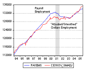
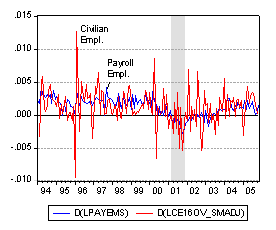
The first figure shows the two employment series (the smoothed and adjusted civilian employment series only begins in 1994), with payroll employment in blue and civilian employment in red. The second figure shows the first difference of the two logged series. As is evident, the variability of the population based series is substantially larger than that of the establishment based series. Over the 1994m01-2005m11 period, the standard errors of the annualized growth rates of the monthly employment levels are 0.00138 versus 0.00284 for establishment and population, respectively. That means that the latter is about twice as variable as the former. (Interestingly, the “drift” terms are about the same, with the implied annualized monthly growth rates equal to 1.5% in both instances).
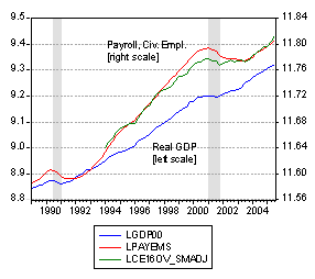
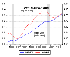
One reason to be interested in employment is to see how it links up with measures of real activity. In the next figure, the two measures are plotted against real GDP, in blue (payroll in red, civilian employment in green, all series now logged). The last figure is hours worked and real GDP, over a comparable period. One would be tempted to do some “ocular regressions” to determine which series is more informative regarding real GDP, but that would lead to differing interpretations. Instead, I decided to characterize the data statistically.
First, all series fail to reject a unit root null (allowing for constant and trend) according to a standard augmented Dickey-Fuller test (where the lag length is selected using a Bayesian information criterion). That means all the series seem to be integrated of order one. One implication of these findings it that it is inappropriate to conduct inference on any of these series using deterministic time trends to “detrend” the data (this is also true for payroll employment over a longer sample, 1950m01-2005m11).
Second, over the 1995q1-2004q4 period (in all subsequent statistical analyses, I have truncated the sample at end-2004 to minimize the effect of data revisions), payroll employment appears to be cointegrated with real GDP, at the 10% marginal significance level, using a maximum likelihood approach (allowing for a constant in the cointegrating equation and a constant in the VAR(4), which is like allowing a deterministic time trend in all of the variables). similarly hours worked is also cointegrated with real GDP, at even higher levels of significance.
Third, the smoothed and adjusted civilian employment series, based on the household survey, does not appear to be cointegrated with real GDP, even at the 10% marginal significance level. Using finite sample critical values would make the failure to find cointegration even more marked.
Fourth, extending the sample back far enough to 1968, both payroll employment and the unadjusted civilian employment series (the adjusted series begin in 1994), as well as the hours worked, are borderline cointegrated with real GDP, but with the wrong sign and statistically insignificant coefficients.
Fifth, since the series are all integrated, it makes sense to examine in addition the information content of the log first-differenced series. Without taking a stand on causality, one approach to doing this is to use principal components analysis, applied to real GDP, payroll employment, adjusted civilian employment, and hours worked. This methodology identifies the vector that minimizes the variance of a linear combination of the variables. The first principal component accounts for 68% of the variation; the series with the highest coefficient is payroll employment, the series with second highest is hours worked, followed by adjusted civilian employment and finally real GDP. A similar result obtains if GDP is dropped from the group; then the payroll series has the highest coefficient.
Sixth, little of this analysis speaks directly to the issue raised by Tim Kane regarding real time analysis. In order to address this issue, somebody (with some spare research assistant resources) would have to use the different vintages of data, such as that available at the
Philadelphia Fed
My conclusion is not that one should only pay attention to payroll employment. Clearly, all the series have information content. Rather, that each series has different characteristics. However, if I had to choose one series, I would still choose the payroll employment series.
Menzie –
This is brilliant, and I really appreciate it. Posts like this are why the whole notion of blogging has such educational power. I for one, learned a great deal here and look forward to any other comments and discussion.
I am a little skeptical about using GDP cointegration alone to judge what is really happening with these two variables. Regarding real-time assessments, note that in some 15% of cases the initial payroll estimate is revised by sign. For example, Sept 05 was initially reported as a -35,000 payroll job loss (to great fanfare), but now is listed by BLS as a 17,000 job gain. Some other observations:
1. The high variance of the household series is no surprise, of course, and is driven by sample rotation, not sample size. CPS found that rotating the household sample is necessary, or else respondent fatigue tends to dull the results. One wonders whether there is some level of respondent fatigue in personnel offices that complete the payroll survey month after month, year after year.
2. My fundamental concern with using payroll data as a barometer for employment is that it is demographically baised. Think of it this way: what would happen to all your series in a country with zero population growth? We would agree that GDP would continue to grow, but payroll employment would be realtively flat, as would civilian employment. The unemployment rate, however, would probably show a tight relationship with GDP. Some analysts are committed to using E-POP or Participation rates, but those, too, are demographically biased for different reasons (labor-leisure choice, age, health, baby booms).
3. I fundamnetally wonder why the media emphasizes payroll employment, and my own theory is that it was successfully driven by the Clinton campaign and presidency (92-2000), when payroll employment was extraordinarily sensitive (weak during the campaign, then superb afterwards). Memory serves that the media emphasized unemployment much more than payroll prior to 1992, after which the Clinton campaign marketed the “jobless recovery” and “discouraged worker” stories so effectively. This isn’t a conspiracy theory, just admiration for good marketing. But the question for economists is how to assess the labor market’s health, and I have yet to be convinced that short-term payroll is even close to the usefulness of the unemployment rate.
Tim Kane: Thanks for the compliment. I tried to be as comprehensive as possible without going into peer-reviewed mode. I agree that cointegration alone should not be the sole reason for focusing on one particular indicator versus another (which is why I also used factor analysis on the first differenced series as well).
As I mentioned, real time analysis would probably imply different weighting systems. When I was at CEA, I recall — perhaps incorrectly — that there too we stressed payroll employment over the civilian employment series because it was viewed as more reliable. Of course, from our discussion, it might depend over what portion of the business cycle one is concerned with. For instance, John Kitchen is focused on the period right after the trough, while
Chauvet and Hamilton (NBER WP 11422) focuses on business cycle dating. In contrast, Chauvet and Piger, St. Louis Fed WP 2005-021A and Evans(NBER WP 11064) rely on payroll employment for business cycle dating). Similarly, for “nowcasting” the economy, Giannone, Reichlin, and Small , FEDS WP 2005-42, employment seems to be the preferred measure.
Clarification to last posting: Kitchen, and Chauvet-Hamilton rely on civilian employment, while the others rely on payroll employment.
Dr. Chinn
The 1990-2000 time frame featured a massive amount of tech r&d and while we had great growth in sales from companies such as Intel and Microsoft, there were a million (exaggeration I hope) start ups that never generated any sales but did have substantial venture capital funded payrolls. Might we suppose that this abberation in economic activity generated much of the divergence between the GDP growth and payroll growth?
Bill
I think that there were two stories that unfolded in the 1990s. A continuing increase in peace and prosperity for the base economy superlaid with a huge waste of capital in the dotcom boom.
Happy New Year to All! Thanks to everyone for their insightful comments.
Bill Ellis: I agree the dot.com boom may have distorted the relationship between payroll employment and GDP. But the puzzle also extends to the slow growth of employment in the wake of the 1990-91 recession. So one question might be whether there something new in the last two decades in terms of the nature of shocks, the composition of the US economy, or the nature of the policy response. Or is the even slower employment growth during the current episode due to different forces than the last recession.
Anonymous presents a related hypothesis. There’s no doubt that a lot of the startups did not continue. But, as the literature on the development of general purpose technologies has pointed out, it may be that a lot of failed startups was necessary in order to find the correct uses for electricity (or internet technologies…). I’m not arguing this is necessarily the case — merely that “waste” is hard to assess.
Do you know where to go on the internet to find corporate capital expenditure trends? (by year and by type).
I used real private fixed investment from the BEA – does this work as an estimate for corporate capital expenditures?
Nate: I’m afraid I don’t have an idea of where you could easily get an aggregate corporate capital investment series. If you had access to some of the proprietary corporate data bases, you could aggregate the individual firm level data. The BEA series should probably include non-corporate investment.
My former CEA colleague, Steve Braun, has a very thorough, and illuminating, analysis of potential reasons for the discrepancy between the payroll and household series:
Steven N. Braun, Reconciling Employment Growth from the CPS and CES, presentation at NBER Labor Studies meeting, April 2004. I highly recommend it as required reading for anybody interested in this issue