Here’s another installment in a series attempting to move the discussion from “my estimate vs. your estimate” (or “prior”, as the case may be) [1] [2] [3] [4] [5] [6] to something more constructive (and hopefully more nuanced). From the conclusion to “Expectations and Fiscal Stimulus” by Troy Davig and Eric M. Leeper:

This paper has embedded estimated Markov-switching rules for U.S. monetary and fiscal policy into an otherwise conventional calibrated DSGE model with nominal rigidities to deliver some quantitative predictions of the impacts of government
spending increases. When monetary and fiscal policy regimes vary — from active monetary/passive fiscal to passive monetary/active fiscal to doubly passive to doubly active — government spending multipliers can vary widely. An increase in government spending of $1 in present value raises output by $0.80 in present value under
[Active Money/Passive Fiscal] AM/PF, while it raises output by as much as $1.80 in present value when monetary policy is passive. In our simple model, this translates into a decrease in consumption of $0.20 in present value under AM/PF, but an increase in consumption of about $0.80 in present value under passive monetary policy.

The paper also simulates the general equilibrium impacts of the government spending path implied by the 2009 American Recovery and Reinvestment Act. When the government spending path is modeled as a sequence of shocks to spending, the present-value multiplier for output is about $0.68 under a fixed regime of AM/PF,
while it can be well over $3.00 in a fixed [Passive Money/Active Fiscal] PM/AF regime. If the government spending path is treated as foreseen by economic agents — because the path is announced by
the passage of the Act — the present-value multiplier for output falls somewhat when the regime is AM/PF, but it rises to nearly $5.00 in the short run when policy obeys a PM/AF regime.

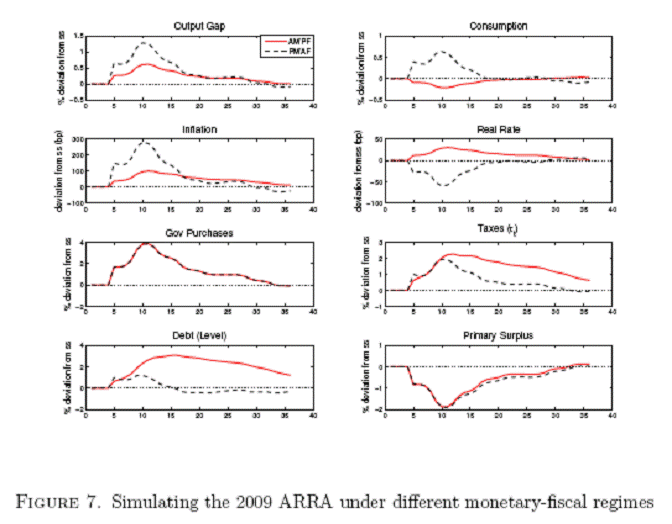
The evolution of the output gap under either regime is shown in Figure 7 from the paper.

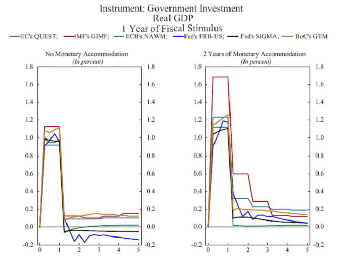
The difference in results depending upon the form of monetary policy is, not surprisingly, not specific to this model. An IMF Conference on Fiscal Policy a couple months ago also highlighted this fact. Particularly salient in this regard was this presentation by Doug Laxton which showed impulse response functions (IRF’s) for a variety of calibrated DSGE models. Below is one example of IRFs for one year fiscal stimulus in the form of government investment, when there is no monetary accomodation, and when there is 2 years of monetary accomodation (I’ll let readers determine what they think is a more realistic appraisal of current monetary policy).

The models’ IRF’s depicted in the graphs are European Commission (QUEST), International Monetary Fund (GIMF), European Central Bank (New Area Wide Model), Board of Governors of the Federal Reserve System (FRB-US and Sigma), and the Bank of Canada (GEM). (The OECD model results are not shown in this particular graph).

Bottom line: The diversity of views regarding multipliers is not always driven by the type of models (although that’s definitely part of it), but can also be driven by assumptions regarding the nature of monetary policy.

Zero interest rate bounds are yet another dimension to be examined. See large multipliers in Christiano, Eichenbaum and Rebelo, who ask “When is the Government Spending Multiplier
Large?” (Their answer: When the zero bound on nominal interest rates is binding.)

Technorati Tags: multipliers, recession,
monetary policy, zero interest bound.