Deficit Hypocrisy Watch
The WSJ editorial page last Thursday remarked upon:
“…the worst fiscal record of any President in modern times…”
Indeed, there has been a point in time when the Federal budget deficit, adjusted for how tax revenues and transfers responds to the state of the economy (what students in my undergraduate course are learning are called “automatic stabilizers”), hit a then record 4.4% as a share of potential GDP! That was in 1986Q3, and the president, as I recall, was Ronald Reagan.
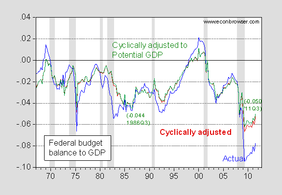
Figure 1: Federal budget balance as a share of GDP (blue), cyclically adjusted Federal budget balance as a share of GDP (red), and cyclically adjusted Federal budget balance as a share of potential GDP (green). NBER defined recession dates shaded gray. Source: CBO, Budget and Economic Outlook, January 2012 automatic stabilizer spreadsheet, and BEA, 2011Q4 advance release, NBER, and author’s calculations.
The WSJ conveniently plotted only the blue line; for a summary of fiscal stance, the red or green lines are better. So, while the corresponding figure in 2011Q3 at 5% is larger in absolute value, it’s only so by about half a percentage point. However, I don’t recall corresponding cries from the Wall Street Journal in 1986. (Oh, and the output gap in 1986 was -0.5 ppts; it was -5.1 ppts in 2011, which I think could account for the additional stimulus. And while I’m at it, note the -2.7 ppt cyclically adjusted budget balance when the output gap was a positive 0.4 ppts (2005).)
Conspiracy at the BLS?
Reader rjs writes in defense of Noel Sheppard’s mis-reading of a BLS release:
… with the benchmark revision & 3 different adjustments, i cannot have confidence in anything in this report…absent the seasonal adjustment, the actual number for january non-farm payrolls was a loss of 2,689,000 jobs; knowing that the BLS confidence interval is on the order of plus or minus 100,000; seasonally adjusting that job loss to show 243,000 jobs gained leaves plenty of room for an error in the methodology…
Since several (usually conservative) commentators (e.g., [0]) have raised questions about the BLS methodologies, I thought it of interest to look at how implausible the estimates are – with a focus on the seasonal adjustment procedure (which seems to be black magic to many). First, here’s graph of the seasonally adjusted and the seasonally unadjusted nonfarm payroll employment series (both easily available to the intellectually curious at the St. Louis Fed’s FRED database, category 11).
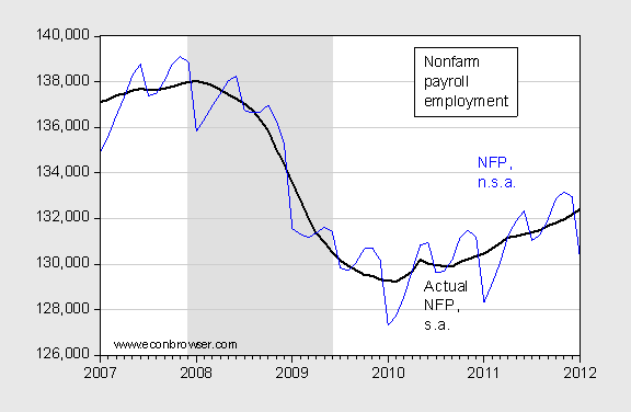
Figure 2: Reported nonfarm payroll employment, seasonally adjusted (black), and not seasonally adjusted (blue), in 000’s, 2007M01-2012M01. NBER defined recession dates shaded gray. Source: BLS January release via FRED, series PAYEMS and PAYNSA, respectively.
So, to the uninitiated it must surely be confusing that the not seasonally adjusted (nsa) series is declining while the seasonally adjusted (sa) series is rising. rjs argues that there is too much going on in the January figures to make anything of the rise. I thought it useful to at least examine the seasonal adjustment process. From BLS:
Estimating Methods
Benchmark data
For the establishment survey, annual benchmarks are constructed to realign the sample-based employment totals for March of each year with the UI-based population counts for March. These population counts are less timely than sample-based estimates and are used to provide an annual point-in-time census for employment. For National series, only the March sample-based estimates are replaced with UI counts. For State and metropolitan area series, all available months of UI data are used to replace sample-based estimates. State and area series are based on smaller samples and are, therefore, more vulnerable to both sampling and non-sampling errors than National estimates.
Population counts are derived from the administrative file of employees covered by UI. All employers covered by UI laws are required to report employment and wage information to the appropriate State workforce agency four times a year. Approximately 97 percent of total nonfarm employment within the scope of the establishment survey is covered by UI. A benchmark for the remaining 3 percent is constructed from alternate sources, primarily records from the Railroad Retirement Board and County Business Patterns. The full benchmark developed for March replaces the March sample-based estimate for each basic cell. The monthly sample-based estimates for the year preceding and the year following the benchmark are also then subject to revision.
Monthly estimates for the year preceding the March benchmark are readjusted using a “wedge back” procedure. The difference between the final benchmark level and the previously published March sample estimate is calculated and spread back across the previous 11 months.
The wedge is linear; eleven-twelfths of the March difference is added to the February estimate, ten-twelfths to the January estimate, and so on, back to the previous April estimate, which receives one-twelfth of the March difference. This assumes that the total estimation error since the last benchmark accumulated at a steady rate throughout the current benchmark year.
Estimates for the 7 months following the March benchmark also are recalculated each year. These post-benchmark estimates reflect the application of sample-based monthly changes to new benchmark levels for March and the computation of new business birth/death factors for each month.
Following the revision of basic employment estimates, estimates for women employees and production and nonsupervisory employees are recomputed using the revised all-employee estimates and the previously computed sample ratios of these workers to all employees. All basic series of employment, hours, and earnings are re-aggregated to obtain estimates for each sector and higher level of detail. Other derivative series (such as real earnings and payroll indexes) also are recalculated. New seasonal adjustment factors are calculated and all data series for the previous 5 years are re-seasonally adjusted before full publication of all revised data in February of each year. [emphasis added – mdc]
In general, one should consult the documentation if one has questions about the NFP series.
Once one has a handle on how the series are created, one can evaluate how sensitive the estimates are to differing approaches. Now, the BLS documentation makes clear the seasonal adjustment procedure is applied to components of aggregate employment, and I don’t have ready access to the n.s.a. versions of the components. But we can still apply the seasonal adjustment process to the aggregate n.s.a. series. Below, I report results when I apply the procedure to a series including and excluding temporary Census workers.
Built into many time-series statistical packages is the standard seasonal adjustment procedure, Census X-12 ARIMA.
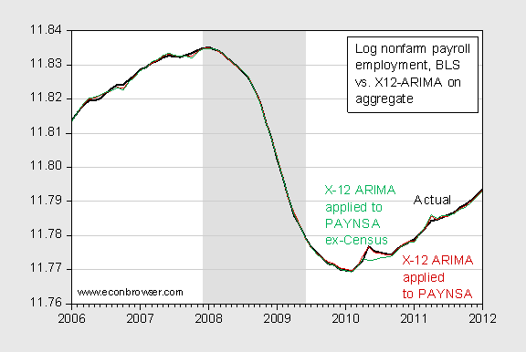
Figure 3: Log nonfarm payroll employment, seasonally adjusted by BLS (black), seasonally adjusted using X-12 ARIMA applied to PAYNSA over 2006-2012 (dark red), applied to PAYNSA ex.-temporary Census workers (green). NBER defined recession dates shaded gray. Source: BLS January release via FRED, series PAYEMS and PAYNSA, respectively, NBER; X-12 ARIMA executed in EViews 7.
To see if these results were driven by the Census procedure, I used a generic seasonal adjustment procedure which estimates seasonal factors as deviations from a moving average (the seasonal factors are assumed to be additive, given I am working on log series). I also estimate the seasonal on differing samples: 1967-2012M01, 1987-2012M01, 2007-2012M01, and the latter, using a n.s.a. series excluding temporary Census workers.
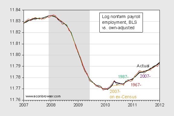
Figure 4: Log nonfarm payroll employment, seasonally adjusted by BLS (black), seasonally adjusted using difference from moving average over 1967-2012 period (dark red), over 1987-2012 period (green), over 2007-2012 period (purple), and over 2007-2012 period on series excluding temporary Census workers (orange), in 000’s, 2007M01-2012M01. NBER defined recession dates shaded gray. Source: BLS January release via FRED, series PAYEMS and PAYNSA, respectively. Additive seasonal executed in EViews 7.
As is obvious from Figures 3 and 4, I do not obtain drastically different results when I apply X-12 ARIMA to the aggregate n.s.a. series, or apply a generic adjustment procedure to a sample starting in 2007. In terms of changes in 2012M01, I find the BLS estimate of 243 thousand to be bracketed by 203 thousand (X-12 applied to PAYNSA) and 282.3 thousand (additive seasonal applied to ex.-Census PAYNSA).
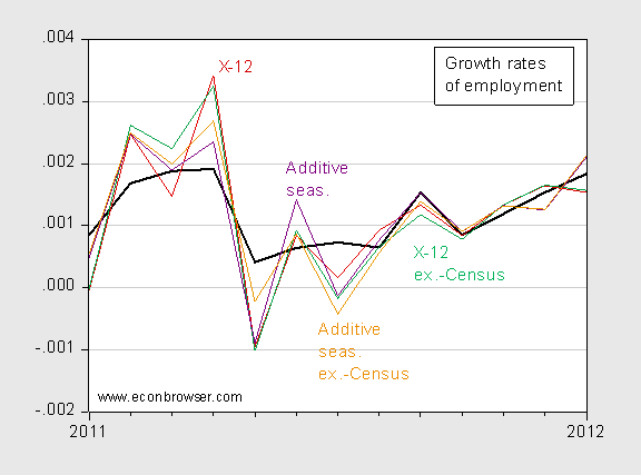
Figure 5: First difference of log nonfarm payroll employment, seasonally adjusted by BLS (black), seasonally adjusted using X-12 ARIMA applied to PAYNSA over 2006-2012 (dark red), applied to PAYNSA ex.-temporary Census workers (green), seasonally adjusted using additive seasonal factors estimated over 2007-2012M01 period on PAYNSA (purple), on PAYNSA ex.-temporary Census workers. NBER defined recession dates shaded gray. Source: BLS January release via FRED, series PAYEMS and PAYNSA, respectively, NBER; X-12 ARIMA and seasonal adjustment executed in EViews 7.
Finally, as I illustrated in Figure 1 of this post, the household series, adjusted to conform to the nonfarm payroll employment concept, which conservative commentators had urged the BLS to construct, evidences a similar upward trend (and has recorded figures consistently higher than the official establishment series. This is something no one else has remarked upon, to my knowledge.
So, there might be some conspiracy in the bowels of the BLS, busily and deliberately churning out misleading employment data, as some conservative commentators suggest. But for me, a little investigation leads me to doubt that thesis.
Wisconsin Coincident and Leading Indicators Pointing Down (Still)
As I noted in a previous post, Wisconsin stood out as one of the few states with negative economic activity trends, starting with implementation of the Governor’s new budget in June.
The Philadelphia Fed’s leading indices indicate that there is little prospect that such trends will reverse. Given the Contractionary policies implemented in the budget [1], this is no surprise.
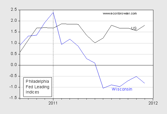
Figure 6: Leading indices for Wisconsin (blue), and for US (black). Dashed line at 2011M01. Source: Federal Reserve Bank of Philadelphia, February 2 release.
To see how remarkable the outlook for Wisconsin is, see the Philadelphia Fed’s map of trends.
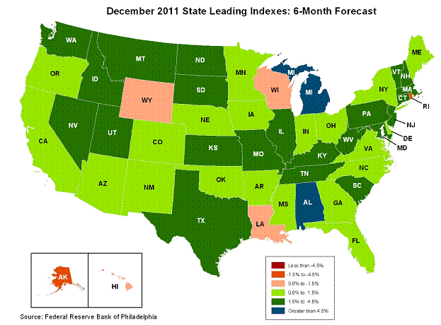
Figure 7: Map of leading indices for December. Indices are forecast for growth rate of coincident indices over next six months. Source: Federal Reserve Bank of Philadelphia, February 2 release.
Wisconsin also stands out in terms of current trends in economic activity (see here and here).
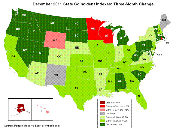
Figure 8: Three month trend in coincident indices. Source: Federal Reserve Bank of Philadelphia, “State Coincident Indexes: December 2011” (January 26, 2012).
Update, 3:45PM Pacific: From WisPolitics Budget Blog this morning:
The Legislative Fiscal Bureau said today the state is now facing a gross deficit of $143.2 million for the 2011-13 biennium, a difference of almost $216 million from past projections.
The LFB said a number of factors combined to worsen the state’s fiscal outlook, including a $272.8 million drop in projected tax revenues through June 30, 2013. The agency noted the projected shortfall exceeds the trigger requiring the guv to submit a budget repair bill and says the administration is discussing steps to address the deficit, including debt refinancing and restructuring.
Gov. Scott Walker said in a statement when compared to other states “Wisconsin is headed in the right direction” and that his administration is “confident in our ability to manage the Wisconsin taxpayer’s money well.” The statement did not offer any steps the administration may take to address the shortfall. Rather, it focused on the LFB projection that the state would end the current fiscal year with a positive gross balance and compared Wisconsin to other states and referenced actions by Walker’s predecessor without mentioning Jim Doyle by name.
“We’ll keep our budget balanced without the job-killing tax increases implemented in the years before we took office; tax increases that led to over 150,000 Wisconsinites losing their jobs in the years before we took office,” Walker said. “In contrast, we’ve added thousands of jobs this year, have the lowest unemployment rate since 2008, lowered the tax burden and will end the year with a surplus.”
Update, Friday 2/10, 11:30PM Pacific:: Readers rjs and tj insist that the January 2012 seasonally adjusted nonfarm payroll number is distorted by the exceptional snowfall in winter 2009-10 combined exceptionally mild winter 2011-12. To see how much this affects the annual growth rates, I compare the log-differenced s.a. and n.s.a. series.
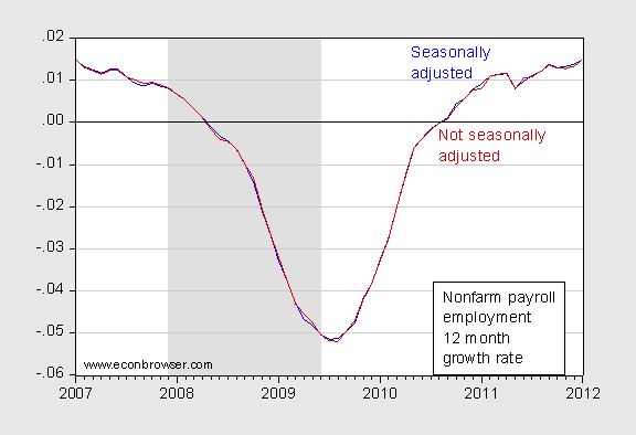
Figure 9: Annual growth rates in seasonally adjusted nonfarm payroll employment (blue), and in not seasonally adjusted nonfarm payroll employment (red), both calculated as 12 month log differences. NBER defined recession dates shaded gray. Source: Source: BLS January release via FRED, series PAYEMS and PAYNSA, respectively, NBER, and author’s calculations.
If you can see a difference for the2012M01 observation, please tell me. (The 12 month growth rate for PAYNSA is 1.5% compared to 1.49% for PAYEMS.)
Update, 2/12, 3PM Pacific:
Reader Jeff criticizes me for concluding that just because the state of Wisconsin is cutting state expenditures (including state and local government employment) that output should fall; apparently, in his mind, it’s just a coincidence that government employment and activity should both start declining with the beginning of the new budget year. To examine this issue a little more closely than in Jeff’s critique, assume Wisconsin economic activity is driven by US economic activity (as assumed in the state government’s Wisconsin Economic Outlook), and state government expenditures. Further assume the latter can be proxied by state government employment:
yWI = f(yUS, gWI)
Run a regression of log Wisconsin coincident index on log US coincident index and log Wisconsin government employment ex.-Federal workers, on a quarterly basis, 2008Q1-2011Q4. Allow an AR(1) correction so that the residuals are not serially correlated at the 10% msl, using Q-statistic (12 lags).
yWI = -7.01 + 0.98 yUS + 0.54 gWI + 0.0000 time
AR(1) = 0.64. Adj. R2 = 0.98. n = 16, 2008Q1-11Q4. SER= 0.002.
The actual, and fitted values using the estimated relationship, and assuming Wisconsin government exployment ex.-Federal held constant at 2011M07 levels for 2011Q3-11Q4 is shown in Figure 10. The implied reduction in economic activity as proxied by the coincident indicator is 1.8%. Since the elasticity of employment with respect to the coincident indicator is 0.74 over this period, the implied reduction in jobs due to the lower state and local employment is 36,800.
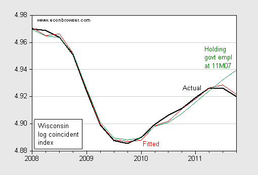
Figure 10: Actual log Wisconsin coincident indices, fitted values and fitted using counterfactual state and local government fixed at 2011M07 levels.
Menzie,
From your graphs and maps it appears that you might want to consider moving to Alabama. Perhaps you could get a job with the Mises Institute at Auburn. LOL!!!
Since you continue to push the hypothesis that state spending cuts leads to lower coincident indexes, do you care to comment on other states that have made significant spending cuts? I believe NV, OR, TX, and WA all fall under this category.
Jeff: Just because I think changes in govenment spending can cause a contraction doesn’t mean that I think the only component of autonomous spending is government spending on goods and services, and transfers (cf problem set 1 in my intermediate macro course!).
And yet when you talk about WI’s coincident index the only thing you cite is changes in government spending. If you feel like there are other important determinants why are they not mentioned? And exactly how did you learn that WI’s lower coincident index is being driven by lower spending and not these other important factors? Cf. any introductory econometrics textbook.
Jeff: Hmm. State and local employment switches direction and starts decreasing in July with the implementation of the new budget. We know from demand determined models that reductions in government expenditures when the exchange rate is fixed often results in contraction. There are modelers who predict job losses [a], and then aggregate private employment declines. Big surprise? I don’t think so, but since I don’t have a fully fleshed macroeconometric model, I can’t fully address your point. But at least I have more evidence than your mere nay-saying. You, on the other hand, have not provided a shred of evidence in favor of your immaculate conception view of the activity drop in Wisconsin.
Menzie, your argument to Jeff relies on correlation? And, correlation = causation?
That’s sad, to ignore the other factors that Jeff simply asked you to delineate/consider.
Menzie, I certainly agree that looking at the budget deficit in cyclically adjusted terms is much better than the raw numbers. How did you do the cyclical adjustment? Is that based on the HP-filter, or did you do something fancier?
menzie, to make note of what you bolded:
New seasonal adjustment factors are calculated and all data series for the previous 5 years are re-seasonally adjusted before full publication of all revised data in February of each year.
my feeling was that the normal seasonal adjustment during the winter months is skewed because it includes the lousier than normal months from the end of 2008 & early 2009:
http://1.bp.blogspot.com/-76fpypjokhs/TyvqffKjTlI/AAAAAAAAMC8/EtV5lLWmt3Q/s1600/BLSPayrollChangeJan2012.jpg
this creates upward bias in subsequent adjustments for those months…
1. I think you can summarize the BLS point as follows: is it rational to believe the BLS is so freaking stupid they would adjust a number once and not see how it flows through their work? It obviously isn’t rational to believe that: that would be an error unacceptable in a college class. The outcry is essentially an argument that the BLS is too dumb to run numbers, which is itself a really dumb argument.
2. Compare Michigan. Unemployment down, running an unexpected surplus. Made cuts, also changed the tax structure, raising taxes on the poor and old while reducing them for the rich. What happened? The auto bailout saved the state. This gets at a point I’ve made in other comments: much of this stuff is marginal and only a little has material impact. People argue about right-to-work or marginal tax rates as though these are magic elixirs when they aren’t. The difference in performance between states that are unionized, that have higher taxes, a bigger safety net, etc. and those that aren’t isn’t regular. There isn’t a clear victory for one side or the other.
People say Texas adds jobs. But California adds more. Massachusetts adds a lot. Low income jobs grow in Texas but high income jobs grow elsewhere. And so on. You can make cases either way. New Jersey only gets back 78 cents of every dollar paid in taxes to DC while SC gets more than a dollar. Why? Mostly because SC is poorer. But SC has been pursuing “growth” policies for decades now. In that time, entire nations have pulled themselves out of poverty – look at Asia – so why is SC still so poor?
CoRev: Yes, in general, one wouldn’t want to blindly equate correlation with causation. Like this crazy statement:
Sounds like this person (i.e. CoRev) is adducing correlation=causation…
Now, at least I have a model, and I can restrict most of the other components of autonomous spending to constant (most exports of WI go to the rest of the US, which was on an upswing (I know you don’t believe that but the data say so), construction investment pretty constant, so G is the only thing we know pretty surely is contracting. I’ll say I’m on stronger ground than Jeff.
rjs,
the winter of 2009-2010 was also the snowiest on record for the east coast. Combine that with one of the mildest winters in 2011-2012 and you have a recipe for garbage in / garbage out.
rjs: Yes, I understand your point; then as I increase the number of years with which I estimate the seasonal adjustment factor, then the impact of the abnormal seasonality you mention is attenuated. That is exactly the point of Figure 4. If I use seasonal factors estimated over the last 24 years (!), I still hit pretty much the implied level as BLS. Only if I use seasonal factors estimated over the last 44 years (over which arguably other things have changed, including importance of agriculture, etc.) do I miss.
Brian: Just used the CBO estimates, reported here.
tj and rjs: See the 12 month growth rates of the BLS seasonally adjusted and the not seasonally adjusted series. If there was such a big distortion due to the effects you mentioned, you would think this would be mitigated in the 12 month changes.
ok, menzie, got it…
Menzie: Lets just be clear what you are doing. Your “analysis” begins with the assumption that a drop in government spending will decrease output. Then to support this position you find the one consistent data point and ignore everything else. And this qualifies as “evidence” in your book?
Menzie,
Well, when I look at nonfarm payroll employment it looks like the end-of-year seasonal drop on payroll employment is lower this year than the last 2 years. There could be other reasons, but we need to see January and February of 2012 as well. If weather is having an impact then the pattern would be bettern numbers for Dec, Jan Feb and worse for Mar, Apr May, after controlling for other variables. It would be intersting to add a time series of temperature/precip to the seasonal adjustment.
Brian How did you do the cyclical adjustment? Is that based on the HP-filter, or did you do something fancier?
The HP-Filter is generally used to detrend data and pull out long cycles. Prescott developed it as a way to mimic the business cycle.
The X-12 ARIMA model used by BLS is actually two models…the regARIMA pre-processor and the X-12 ARIMA seasonality model. regARIMA filters outliers, level shifts, deterministic seasonal factors and trading day effects. The detrending used to be done in the older X-11 version, but with X-12 it was moved to the regARIMA module. It uses a centered Henderson moving average. The X-12 module accounts for nonstationary seasonality issues; e.g., the old “Airline” ARIMA(0,1,1)(0,1,1) w/o constant model is the default. So it will take the first difference of both the nonseasonal and seasonal terms.
You might be interested in Eurostat’s TRAMO-SEATS model used by the European Statistical Office. Most software packages have both X-12 and TRAMO-SEATS, but usually TRAMO-SEATS is in a stripped down version. You can get a complete version here:
http://www.ecmwf.int/research/demeter/
FWIW, I’m currently wrapping up a paper that compares X12 and TRAMO-SEATS using Army rotary wing flying hours, which is highly seasonal.
A couple of good references on X-12 ARIMA and TRAMO-SEATS are: Findley, Monsel, Bell, Otto and Chen, “New Capabilities and Methods of the X-12-ARIMA Seasonal Adjustment Program,” Journal of Business and Economic Statistics, (1998) vol 12, p 299-309
and
The Econometric Analysis of Seasonal Time Series, by Eric Ghysels and Denise Osborn (Cambridge University Press).
It amazes me that even macroeconomists can be left-wing.
I mean ‘left-wing’ and ‘economic fundamentals’ seem to be a virtual contradiction in terms.
Microeconomics makes it impossible to have leftists-redistributionist views on economics. But it appears Macroeconomics is sufficiently academic and detached from day-to-day micro, that there is enough wiggle-room for socialists to reside in the field.
I suspect many Economists are people who covet money, but don’t have much ability to make much of it themselves. Economics is a discipline that can provide haven to socialists.
Menzie, other than being a tad snarky, my comment you referenced re: bill status was derived from the actual House and Senate web sites of the time frame.
So neither correlation nor causation. Just facts! Since then the Senate has passed 1,000 days without passing a budget.
Your own comment: “…construction investment pretty constant, so G is the only thing we know pretty surely is contracting. I’ll say I’m on stronger ground than Jeff.” Leaves an impression that continued deficit spending was preferable to WI overall than getting state spending under control.
I presume that WI, as most states, has a “balanced budget” constitutional requirement thet won onthan when the republicans were elected. Which,
Crap, I hovered too long on the wrong part of the screen.
That was supposed to end with: on which the republicans won the election.
There are important differences between the Reagan and Obama cyclically-adjusted deficits. First a key similarity: both inherited problems of historic magnitude. Reagan’s was stagflation and Obama’s was the final plunge of the Great Recession. Reagan chose to break the back of inflation by a four-plank program that precipitated the 1982 recession. He also chose to ramp up defense spending to (hopefully at that point in time which is the context that must be taken into consideration) bankrupt the Soviet Union and thus bring to an end the greatest threat to our survival – the Cold War. By a wide margin, historians now judge this aspect of Reagan’s fiscal policy to have been a resounding success. By fiscal 1986, the defense buildup had added an additional 1.3 percentage points to the deficit (from the base year of 1980). An arguably more insightful way of making comparisons between Reagan and Obama takes account of this initiative. Similarly, no economist or historian would think of dunning FDR for the record defense buildup during his tenure. Adjusting the 1986 peak Reagan deficit of 4.8% per the CBOs table by this 1.3 gives a more meaningful 3.5%. Obama can claim no comparable need for an adjustment for defense. Each of the four years of the Obama term will have exceeded the Reagan peak by a wide margin, with 2012 projected to come in lowest at 4.3%.
Even more to the point is the full tenure picture for Obama and Reagan. Reagan’s 8-year fiscal record, without making the defense adjustment, was a cyclically-adjusted ratio of 3.3%. Per the CBO, Obama’s 4-year fiscal record will be 5.8%. Moreover, the historical context has changed. The level of debt today is far more pressing on whomever is in office. As for a greater output gap today than back in the 80s, this is (mostly) a moot point as it is cyclically adjusted away. Of course we could look at a triple-adjusted deficit series: cyclical, temporarily-necessary-defense, and something to account for some additional part of today’s deficits that should not be charged to Obama. But until such an empirical series is created, the above is what we have to go on. The Wall Street Journal, no matter what you think about their editorial policy, has this one right.
JBH: “Reagan chose to break the back of inflation…” And here I thought that Fed Chairman Volcker had something to do with it. Silly me. Even more silly of me to think that tax cuts and increased government spending would tend to push up the price level rather than depress it. I will have to acquaint myself with the alternate reality which constitutes your universe.
JBH What would you and the WSJ prefer? That Obama not run large deficits? If you want to criticize Obama’s economic policies, then I think you’re on firmer ground if you criticize him for being too concerned about short-term deficits.
But your history needs some corrections. No one would be arguing for large fiscal deficits if the Fed were not at the zero bound. The Reagan recession was created by the Fed and cured by the Fed. The Fed could do this because we had very high nominal interest rates, so there was a lot of room between reality and the zero bound. A better question is to ask why Reagan chose to run large deficits when monetary policy was still a viable alternative.
You also fumbled the ball with your defense comments. First, DoD budgets would have gone up in the 1980s regardless of whether Carter or Reagan won in 1980. In fact, in his last two budgets Carter already increased DoD spending quite dramatically. During the 1970s readiness of conventional weapon systems was low because DoD was trying to maintain older pre-Vietnam era weapon systems at the same time they were trying to do R&D work on “Force Mod” systems. That R&D work started in earnest under Gerald Ford. By the time Carter left office many of those systems were just starting to be fielded. Reagan inherited a situation in which a lot of systems started by Ford & Carter were just coming online or moving out of the early stages of the “provisioning” stage of DoD’s life-cycle model. Examples include the F-14, the F-15, the Nimitz class aircraft carrier (recall that Carter compelled the Navy to order more Nimitz carriers), the B1, the M1 Abrams tank, the Bradley Fighting Vehicle, the Paladin self-propelled howitzer, the M198 towed howitzer, the Multiple Launch Rocket System, the Patriot missile system, the UH-60A Blackhawk, the AH-64A Apache, Pershing II theater nukes, etc. In fact, just about every major weapon system that makes up the backbone of today’s DoD was developed under the Ford and Carter administrations and brought online just as Reagan came into office. This put a lot of stress on the budget because there was a period of ~10 years when new systems had to be deployed at the same time older systems had to be supported. So Army had to support both the M1 Abrams and the pre-Vietnam M60 tank and the pre-Korean War M48 tanks. Army had to support both the Bradley vehicles and the M113 personnel carriers. Navy had to support both older Poseidon and newer Trident submarines. Air Force had to support Cuban missile era Titan II missiles, 1970s era Minuteman III missiles, and the new MX missiles. The fact is that DoD budgets in the 1980s would have been pretty much what they were regardless of who was President.
And this bit about Reagan wanting to run big defense budgets because he felt it would bankrupt the USSR is a complete fiction made up after the fact. What bankrupted the USSR were the bags of rubles that they had to send to Cuba, Hungary and Poland in the early 1980s. Those transfers far outweighed any increased defense burden on the USSR. And those payments also represented leakages from the USSR economy; something that increased defense spending did not represent. If you want to credit someone with bringing down the USSR, give credit to the Pope and the Gdansk shipyard workers.
Finally, even if one agrees with your claim that Reagan’s defense budgets were wise and necessary at the time, that is not in-and-of-itself a reason why those defense budget increases had to be financed with structural deficits. Why is defense spending exempt from the normal budget principles of having to raise taxes if you want to structurally increase spending?
Jeff: I have posted what I have found at the end of the post. Perhaps you can get more data than I can get at a high frequency, and model Wisconsin’s economy in a more sophisticated fashion — I’ll post it if you actually do the work and send it to me. Not that I’ve seen anything constructive from you in the past.
2slugbaits,
Sorry, you are wrong. Reagan certainly thought he was out to bankrupt the USSR. He was wrong in that, but you are also wrong that it was leakages to Cuba et al that did them in. The combination of a stagnating rate of growth due to a failure to introduce ongoing technological changes in the economy combined with the sharp decline of oil prices in 1986 (that pretty much stuck) were the main factors, along with the political crisis that erupted in 1989-91 by states and republics wanting to get out of Russian domination within the CMEA. After all, the big economic collapse came after 1989 and was across the whole zone.
Barkley Rosser I don’t think you’ll get any argument from me about stagnating growth in the USSR and the collapse of oil prices. Those were certainly important factors. My point is that the supposed stress that Reagan’s defense build-up put on the Soviet economy is way overblown. In fact, most estimates I’ve seen show that while the USSR did increase defense spending in the late 70s and early 80s, by the mid-80s (i.e., the so-called “Star Wars” period) Soviet defense spending had already leveled off. So you have to look pretty hard to find this supposed increased stress given that Soviet defense spending did not actually increase as a percent of GDP after the early 1980s. So the timing just doesn’t work. But the explanation that does work is the stress created by the Warsaw Pact countries’ demands for more “Ghoulash Communism” and Gdansk Agreements for everyone. After the Soviets caved and agreed to the Gdansk Agreements the game was up. The Agreements gave Polish workers the power to demand very large wage increases, which had to be subsidized by the Soviets. And soon workers in the other satellite countries started demanding the same benefits. Even Cuba was up to $2B/year. For example, food prices increased 40% after the Gdanks agreements, and under the Council for Mutual Economic Assurance (CMEA) protocols it was the Soviets who had to make up the shortage. That’s why Gorbachev first allowed perestroika to blossom in the satellites long before he allowed it in the USSR proper. Gorby was trying to get out from under having to support the satellite countries. That allowed the satellite countries to establish mediating institutions.
If you had to pick one thing that was most responsible for the collapse of the Soviet economy, I think you’d have to say it was due to the Gdansk shipyard workers. Yes, the Soviet economy was inherently inefficient, but it had been inefficient for a very long time. Sooner or later it would have collapsed; but absent the Gdansk strikes it probably would have been later.
Pretending that the USSR fell because of Reagan’s Star Wars initiative is something that ingratiating ex-Soviet generals like to tell American generals because they know it’s the kind of thing that flatters American egos. But when it comes to economic matters I don’t listen to ex-Soviet generals anymore than I listen to American generals.
2slugb,
If you read my post carefully, you would see that I agree with you on the matter of defense spending and its (non)-role.
However, I disagree with you on the Gdansk agreements playing much of a role. All that happened in Poland was that they got massive inflation, given that like Hungary (and earlier, Yugoslavia) they had largely dumped command central planning in favor of market socialism. The USSR was not paying their bills for that, they were. There were other CMEA eastern European states that were not pulling that stuff and had less perestroikized policies than did the USSR, e.g. Czechoslovakia and East Germany.