Today we are fortunate to have a guest contribution written by Yuriy Gorodnichenko (UC Berkeley) and Michael Weber (UC Berkeley). It is based upon their paper entitled “Are Sticky Prices Costly? Evidence From The Stock Market”.
We argue that the inflexibility of firms in adjusting prices after nominal shocks is associated with real costs. Employing information in the stock prices of firms, we show that, in a high frequency event study around policy decisions of the Fed, monetary policy shocks lead to a larger increase of conditional volatility for sticky price firms compared to flexible price firms, thus confirming a cornerstone of New Keynesian macroeconomics and offering a justification for active fiscal and monetary policy.
In principle, fixed costs of changing prices can be observed and measured. In practice, such costs take disparate forms in different firms, and we have no data on their magnitude. So the theory can be tested at best indirectly, at worst not at all.
Alan Blinder (1991)
Debates in business cycle macroeconomics are often centered around two questions. First, positively, can central banks influence the real economy? Second, normatively, should central banks do anything to stabilize business cycles? In the context of real business cycle models, the answer is a clear “no” to both questions because purely nominal shocks are neutral (that is, changing money supply does not influence real output) and agents’ responses are optimal so that stabilization policy can only reduce welfare. On the other hand, a central feature of modern New Keynesian models is price rigidity in the short run which leads to inefficient fluctuations in the economy thus calling for stabilization policies. This feature also makes central banks a potent force in the economy as money is no longer neutral when prices are fixed. The contrast between these models is further amplified when one considers their predictions with respect to the size of fiscal multipliers. For example, government spending shocks in real business cycle models strongly crowd out private consumption and investment so that the multiplier is generally small and well below one (that is, a dollar increase in government spending raises output by less than a dollar), while in New Keynesian models the multiplier can be much larger due to price rigidities and other frictions.
Knowing which of these models is appropriate for policy is especially crucial in the current environment of depressed economies and so this is not just an academic debate between different schools of thought in macroeconomics. How can one differentiate between these models? Which of them is a better description of reality and hence a foundation for policy? While there are potentially many tests, it seems that it would be most informative to explore if price rigidities, the fundamental premise of New Keynesian models, are meaningful.
There seems to be a growing consensus that prices at the micro-level are fixed in the short run (Bils and Klenow (2004), Nakamura and Steinsson (2008)), but it is still unclear why firms have rigid prices. A central tenet of New Keynesian macroeconomics is that firms face fixed “menu” costs of nominal price adjustment which can rationalize why firms may forgo an increase in profits by keeping existing prices unchanged after real or nominal shocks. However, the observed price rigidity does not necessarily entail that nominal shocks have real effects or that the inability of firms to adjust prices burdens firms. For example, Head et al. (2012) present a theoretical model where sticky prices arise endogenously even if firms are free to change prices at any time without any cost. This alternative theory has vastly different implications for business cycles and policy (e.g., nominal shocks are neutral and thus a central bank has little if any influence on the economy). How can one distinguish between these opposing motives for price stickiness? Our key insight is that in New Keynesian models, sticky prices are costly to firms, whereas in other models they are not. While the sources and types of “menu” costs are likely to vary tremendously across firms thus making the construction of an integral measure of the cost of sticky prices extremely challenging, looking at market valuations of firms can provide a natural metric to determine whether price stickiness is indeed costly. In a recent paper (Gorodnichenko and Weber 2013), we exploit this key insight using stock market information to quantify these costs and—to the extent that firms equalize costs and benefits of nominal price adjustment—”menu” costs. The evidence unambiguously supports the New Keynesian interpretation of price stickiness.
Specifically, we merge confidential micro-level data underlying the producer price index from the Bureau of Labor Statistics with tick by tick stock price data for individual firms from NYSE Trade and Quote. As a first pass, we sort firms into portfolios based on the frequency of price adjustment and find a premium for holding the portfolio populated by firms with the stickiest prices relative to the portfolio populated by firms with the most flexible prices equivalent to at least 0.3% – 0.8% loss in revenue.
While this summary statistic provides a simple metric, it does not explain how nominal rigidities affect firms at the micro level. To identify a causal effect of price rigidity on stock returns, we use rich cross-sectional heterogeneity of firm characteristics and high frequency stock market data. Our source of variation are monetary shocks identified from futures on the fed funds rates—the main policy instrument of the Fed—in a narrow time window around press releases of the Federal Open Market Committee. We calculate the response of returns for firms with different frequencies of price adjustment over the same narrow window so that we can rule out reverse causality and other aggregate shocks.
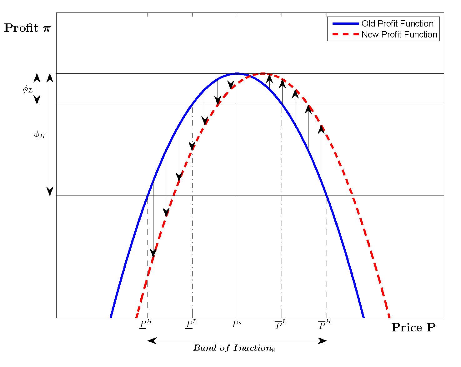
To guide our empirical analyses, we show in a basic New Keynesian model that firms with stickier prices (larger menu cost φ) should experience a greater increase in the volatility of returns than firms with more flexible prices after a nominal or real shock. Intuitively, firms with larger costs of price adjustment tolerate larger departures from the optimal reset price. Figure 1 plots the profit function of a firm in a static New Keynesian model and illustrates this intuition. In response to a shock that shifts the profit function from “old” to “new”, both flexible and sticky price firms might experience an increase or decrease in returns. Hence, looking solely at profits or returns is not sufficient. However, there is an unambiguous prediction with respect to the variance of changes in payoffs in response to shocks: firms with high menu costs (stickier prices) should experience larger variability in payoffs than firms with low menu costs.
Consistent with this logic, we find that returns for firms with stickier prices exhibit greater volatility after monetary shocks than returns of firms with more flexible prices, with the magnitudes being broadly in line with the estimates from a calibrated New Keynesian model with heterogeneous firms: a hypothetical monetary policy surprise of 25 basis points leads to an increase in squared returns of 8%2 for the firms with stickiest prices. This sensitivity is reduced by a factor of three for firms with the most flexible prices in our sample. Our results are robust to a large battery of specification checks, subsample analyses, placebo tests, and alternative estimation methods.
In summary, our results suggest that sticky prices are indeed costly for firms — consistent with the tenets of New Keynesian macroeconomics. While price inflexibility is only one of the key ingredients in many modern macroeconomic models, it can justify policies aimed to stabilize business cycle fluctuations as well as inform us about the design of optimal stabilization policies for central banks and fiscal authorities. Our results are unambiguously consistent with theories calling for active, expansionary fiscal and monetary policy in the current economic environment.
References
- Bils, M. and P. J. Klenow (2004). Some Evidence on the importance of sticky prices. Journal of Political Economy 112 (5), 947-985.
- Blinder, A. S. (1991). Why are prices sticky? Preliminary results from an interview study. American Economic Review 81 (2), 89-96.
- Gorodnichenko, Y., and M. Weber (2013). “Are Sticky Prices Costly? Evidence From The Stock Market,” NBER Working Paper #18860.
- Head, A., L. Q. Liu, G. Menzio, and R. Wright (2012). Sticky prices: A new monetarist approach. Journal of the European Economic Association 10 (5), 939-973.
- Nakamura, E. and J. Steinsson (2008). Five facts about prices: A reevaluation of menu cost models. Quarterly Journal of Economics 123 (4), 1415-1464.
This post written by Yuriy Gorodnichenko and Michael Weber.
“the answer is a clear “no” to both questions because purely nominal shocks are neutral (that is, changing money supply does not influence real output)…”
It looks to me as though real output is back to a normal growth path after having nominal values inflated for many years… “artificially manufactured” if you will.
However, many economists expect to raise real GDP back up to a potential real GDP that existed during the bubble years. This is an error in thinking.
I actually show that we have returned to a normal growth path in real GDP value and also that potential real GDP is below real GDP. The economy is showing dynamics of reaching the end of an expansionary phase of the business cycle.
The main problem we have now is high unemployment. And the cause of that is low effective labor share of income, around 74%. According to my calculations, all we need do is raise effective labor share back to where it was before the crisis, 78%… and we would have enough effective demand to lower unemployment to 6%.
We can call for more active fiscal and monetary expansionary policies, but let’s keep in mind where effective demand is and how it will limit any expansion.
Effective demand was a core principle of Keynes’ work. I have determined an equation for it.
Effective demand = real GDP * els/(cu*(1-u))
els = effective labor share, (0.78*labor share: business sector, 2005=100)
cu = capacity utilization
u = unemployment rate
The denominator is combined utilization of labor and capital.
Here is a graph of the variables (real output, potential real output and also effective demand) returning to a normal growth path.
http://effectivedemand.typepad.com/ed/2013/04/back-to-reality-potential-real-gdp.html
It seems to me this whole argument ignores the role of prices in the equilibrating economic decisions that ultimately raise an economy out of a slump. The question I want to understand first is why are prices sticky? I need this before I want to ask what monetary policy will do to stick prices.
Alchian in “Information Costs, Pricing and Resource Unemployment” (1969) shows that sticky prices have at least one purpose, to lower search costs by stabilizing prices. If every exchange was an auction, buyers would have no idea how much they will spend before attempting to buy a good. One of the “costs” of inflation is uncertainty about future prices.
I’m wondering if I am just one step behind everyone else in the world and you all know why sticky prices are not conveying any information that we should care about and we can ignore their purposes. If not, can someone help me make the jump from concern about the purpose of stick prices to concern about how to eliminate them?
Thanks
@Edward, WRT effective demand and the trend rate of current and potential GDP, note that post-Boomer demographics resulting from the differential of Boomer-Millennial sizes to population and labor force imply that the labor force growth rate will be no faster than 0.5% hereafter; this compares to the long-term avg. of 1.5%, 1.8% at peak Boomer entrance to the labor force, and 1.2% since peak Boomer entrance. Should Boomers leave the labor force sooner and in larger numbers, the labor force growth rate will be slower, perhaps as slow as 0.2-0.3% in the meantime.
Irrespective, the post-Boomer dependency ratio, regressing the slower labor force growth and participation constraints, implies that the US labor force will cease growing altogether by no later than the mid- to late ’20s.
Moreover, the trend deceleration of US labor force growth will be faster than that of Japan since the ’90s, as the US experienced a faster rate at the peak and remained at a higher plateau rate longer. IOW, the Boomer demographic drag effects are likely to be more intense and last at least as long as that which has occurred in Japan since the late ’90s.
Finally, note that the post-’00 trend real GDP and real GDP per capita have slowed from 3.3% and 2.1% to 1.6% and 0.8%, whereas the trend since ’07 has decelerated further to ~0.6% and negative. The once-in-history Boomer demographic drag effects imply post-’00 trend real GDP will continue to decelerate from 1.6% today to 1% or lower by decade’s end, with post-’07 real GDP and real GDP per capita remaining around 0% and more negative hereafter.
Regarding the demographic cycle progression, the US is where Japan was in the early ’00s. Japan has lost an equivalent of 40-45% of real GDP growth per capita since the secular peak in ’89-’90 vs. the long-term trend rate. The US has lost ~25% of real GDP growth per capita, and we are on track to match Japan’s loss of growth per capita by decade’s end.
By any objective measure, this is a Great Depression-like loss of real GDP growth per capita, albeit a slow-motion variety.
As in Japan since the ’90s and the world in the 1930s to before WW II, supply-side tax cuts, reserve bank printing, and Keynesian deficit spending with EXTREME wealth and income concentration, plunging money velocity, and record debt/GDP cannot overcome the secular demographic drag effects that will intensify in the years ahead for the US, EU, and eventually China.
reply to Bruce…
Are you getting these lower growth rates by comparing the present economy to the bubble years? That would not be reasonable, because the value of real GDP has made a correction even in real terms due to the crisis. Did you see the graph I posted above?
Labor force participation does not affect my numbers. You have a labor force and the issue is what % of that labor force can you utilize? The % utilization rate of labor is limited by % labor share of income.
The true issue is the dynamic in the economy that allows the utilization rate of labor to increase. This is the important distinction coming from my equation. It is not an issue of total numbers, but percentage of the number you have. It’s a ratio thing…
There are many who want to push real GDP upwards to who knows where… but if you push on real GDP, eventually you hit the limit of effective demand and start scratching your head, because utilization rates of labor and capital top off. Before the crisis, capacity utilization and unemployment didn’t improve for 3 years. We were at the effective demand limit. (I am talking unemployment rate, not labor force participation.)
The economy looks to have shed itself of the bubble values. Values which were artificially created. We should not go back up there. Real GDP, potential real GDP and effective demand have come back to a long-run real growth path.
When unemployment hit 3.9% in 2000, the forces creating the bubble were in full force. You can look at this graph.
http://effectivedemand.typepad.com/.a/6a017d42232dda970c017ee9fdfba7970d-pi
During Clinton’s 8 years in office, effective demand rose from $9 trillion to $12.6 trillion. That is a huge expansion in effective demand and we saw big job growth from that. During the Bush years, effective demand stayed between $12.6 trillion and $13.4 trillion. It was a time of stagnant effective demand. During Obama’s term, effective demand is only up to $14.2 trillion. You can see that under Clinton, there was job growth, but the bubble that was created ultimately was damaging to the economy. It left behind high inequality, low labor share and high unemployment.
To end, we are back to a normal growth path, and simply need to raise effective labor share back above 78% from the 74% it has fallen too. The solution is that simple to stabilize the economy on its current and correct path.
@Brian – “The question I want to understand first is why are prices sticky?”
Agreed, and I seem to recall that the elder Galbraith had much to say about quasi-monopolies preferring to keep prices sticky (higher) and reduce production and employment, rather than reaching a lower-price, higher-production, higher-employment equilibrium that would be expected in a more competitive marketplace.
The price-stickiness issue is therefore linked to the topic of monopolistic corporations extracting historically-extreme (high) profits as a share of GDP. It’s unfortunate that this post doesn’t address that issue.
Returning to the title question of the original post, the answer is “yes”, we should care.
Regarding their conclusion that sticky prices impose real costs on corporations, I remain skeptical that tests based on stock market returns are meaningful metrics. The key finding that “(short-term? stock market?) returns for firms with stickier prices exhibit greater volatility after monetary shocks than returns of firms with more flexible prices” could have many potential explanations, having little to do with price stickiness, and much more to do with investor perceptions, nature of the business (risk levels, interest rate sensitive financing, sector of the economy, monopolistic vs competitive marketplace, revenue sources, inflation-sensitive supply chains), and so on. The author’s assertions of robustness need to be documented before such a claim can be credible.
Brian Albrecht can someone help me make the jump from concern about the purpose of stick prices to concern about how to eliminate them?
I’m not following you. I didn’t get the sense that the authors were arguing for eliminating sticky prices. In fact, sticky prices are something of a necessary condition for a New Keynesian model. What the authors examined was whether sticky prices were costly to firms. The authors find that they are costly, so presumably there is some good reason why some firms are unable to avoid those higher costs. And while that might be a good thesis topic for some eager young grad student at the Booth School, it really isn’t the point of this paper. Here the authors are undercutting a key tenet of real business cycle theory and finding empirical evidence that supports a New Keynesian perspective. The authors are not trying to find ways to overcome price stickiness; they are simply looking for microfounded evidence that it exists.
This was really interesting. Thanks. I loved the use of the data set.
@Edward, thanks for the thoughtful and reasoned reply.
Looking at data from the late 1960s is insufficient to capture the long-term trends in real GDP per capita. I contend that we have experienced a regime switch in the ’80s-’90s to a log-linear constraint to real GDP per capita similar to that which occurred from the 1870s-90s to the 1920s. A log trend since the ’80s is more appropriate than an exponential trend.
http://arxiv.org/ftp/arxiv/papers/1205/1205.5671.pdf
http://www.voxeu.org/article/us-economic-growth-over
http://www.forbes.com/sites/haydnshaughnessy/2013/02/01/is-it-the-end-of-growth/
http://www.investmentnews.com/article/20121120/FREE/121129995
http://www.bloomberg.com/video/investment-strategist-jeremy-grantham-rBP3CUZJS9mPRsuWLXpSRA.html
Long-term real GDP per capita is a linear function WRT population. Each regime switch occurred in the past at a higher punctuated log-linear equilibrium bound based on emergence of a new techno-economic/energy epoch, if you will, e.g., wood to coal to oil to the cumulative coal, oil, and nuclear (and now solar, wind, etc.) to produce electricity and heating, transport, and industrial fuels. The energy epoch since after WW II permitted exponential growth until the growth of debt grew at a super-expential rate beginning in the ’90s into the ’08 crash.
However, this time around, unlike the 1880s-1900 and 1930s-50 when the constant-dollar price of oil was in the $20s-$30s and land and infrastructure costs of build out and maintenance were comparatively low, oil priced in the $90s-$110 due to peak global crude oil production per capita will now exert a long-term log limit bound constraint to real GDP per capita and population rather than permit a resumption of exponential growth of real GDP per capita hereafter.
US population and labor force growth will (is) decelerate (decelerating) to a rate of half or less the long-term avg. Absent a productivity shock that also includes more employment than is displaced, which looks unlikely at this point, the speed limit for US real GDP per capita since the regime switch and onset of the debt-deflationary regime will be around 0% hereafter, exacerbated by energy constraints and the Boomer demographic drag effects.
Therefore, “potential real GDP” will be much slower than CBO and conventional economic models anticipate, which will have an unexpectedly severe and lasting effect on tax receipts and fiscal budgets, gov’t spending per capita, pension underfunding and payouts to retirees, employment, wages, profits, private investment, stock and real estate prices, etc.
The return to real GDP and real GDP per capita growth rates of 3% and 2% is highly unlikely.
I would add to above that regressing the log of productivity with labor force/population given the Peak Oil/post-Oil Age energy regime (persistence of total oil consumption at or above 4% of GDP) suggests a trend productivity of no faster than 0.3-0.4% and labor force/employment and population growth of no faster than 0.4-0.5% and 0.6-0.7%, implying real GDP per capita of effectively near 0%.
Using ~0.7-0.9% as the “potential real GDP” trend rate, rather than CBO’s 2.4%, implies that there is essentially no output gap.
About 3.3% of the incremental nominal growth of GDP since after WW II and the early ’80s was associated with debt-money inflation to wages and GDP. This nominal growth factor multiplier will not exist hereafter, which implies a trend nominal GDP rate around 1.7% and 1% or slower per capita.
Wage growth will thus be capped at 2% or less (less for the bottom 90% because of skew to the top 10%) without additional capacity expansion, which is not suggested because of constraints from energy costs/GDP and slow growth of the labor force.
Boomer demographic drag effects will result in a once-in-history shift in the composition of household spending from high-multiplier expenditures for housing, autos, and child rearing to low-multiplier outlays for house maintenance, property taxes, utilities, and out-of-pocket costs for insurance premia, coinsurance, medical services, and medications.
“Second, normatively, should central banks do anything to stabilize business cycles? In the context of real business cycle models, the answer is a clear “no” to both questions because purely nominal shocks are neutral (that is, changing money supply does not influence real output) and agents’ responses are optimal so that stabilization policy can only reduce welfare.”
That’s quite a mouthful! I would say that it depends on what you call central bank stabilization. From my perspective, the central bank’s most important function is to control CREDIT. When it allows Total Credit to mushroom to several times GDP, conditions are ripe for credit default and financial crisis.
Caution should be the by-word when addressing interests that profess that “stabilization policies can only reduce welfare”. These market forces might support continual laissez faire expansion of credit and ineffectual governance of banking and finance.