Consider the following graph, with both series (coincident series for economic activity) normalized to 2011M01=0.
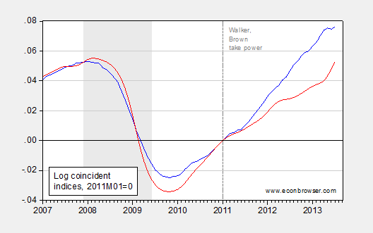
Figure 1: Log coincident economic indexes, both normalized to 2011M01=0. NBER defined recession dates shaded gray. Source: Philadelphia Fed, NBER, and author’s calculations.
One series pertains to the state I live in now (Wisconsin), and has pursued a policy of spending cuts and tax cuts skewed towards high income groups. The other is the state I lived in before coming to Wisconsin (California). It dealt with the serious fiscal problems it faced in part by cutting spending, and by raising taxes. Interestingly, both states had new governors taking power in January 2011 (Walker in Wisconsin, Brown in California). And in both cases, one party holds power in both houses of the legislature, as well as holding the governorship — Republicans in Wisconsin, Democrats in California.
It’s not surprising to anybody with acquaintance with data (or just plain reality) that the red line is Wisconsin, the blue is California. While this is not a controlled experiment — there are many other variables of importance (although they both share the same monetary policy) — the comparison is suggestive.
So, for completeness’s sake, here is the figure again, series labeled, and the US series added.
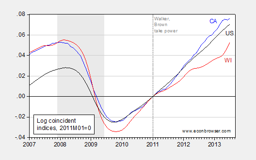
Figure 2: Log coincident economic indexes for California (blue), Wisconsin (red), and US (black), all normalized to 2011M01=0. NBER defined recession dates shaded gray. Source: Philadelphia Fed, NBER, and author’s calculations.
More on California here.
Imperial military neo-Keynesian fiscal policy will be dominated by imperial war spending (and profiteering) and “self-sacrifice” and “austerity” for the bottom 90% in the years ahead as the imperial war cycle repeats and the last-man-standing contest for the remaining scarce resources on a finite planet intensifies.
Get ready for 9/11 II, only this time the scale must be far larger owing to the imperial war- and “recovery”-weary American public’s lack of enthusiasm for more mass death and destruction at their expense in terms of employment, after-tax wages, purchasing power, medical services, and overall financial, economic, and psycho-emotional well-being.
War is the business of empire, and war is good business.
If you crunch the numbers using the leading indexes from the philly fed you will see that Wisconsin is expected to grow much faster than average in the coming months. Cali and Wisconsin’s log coincident index will be nearly equal to the US average by the beginning of next year according to the leading indexes.
US:0.035212
Wisconsin:0.03428
Cali:0.0358
Do you have any comments on this Menzie?
I should note in my last post I used log10, I see you used ln. Doesn’t change much though. So the numbers on your chart in 6 months are expected to be:
US: 0.081079023
Wisconsin: 0.078931761
Cali: 0.082485477
Curious. So our take is to be that lowering government spending and raising taxes is stimulative? By the way, are the amounts of spending cuts, etc. normalized as well?
Not sure what you’re trying to do here.
California is much more dependent on real estate, construction, and the wealthy than Wisconsin.
Its recovery is much more about Bernanke reflating the real estate and equity bubbles than about anything Brown did.
If Wisconsin had more million-dollar homes and tech industry stock-option millionaires, its recovery would be more like California’s.
Professor,
I would refer you to the recent post by your fellow blogger Professor Hamilton entitled “Geography of Success”. I dont believe there are dates attached to map he includes but given the color scheme Professor Hamilton employed it appears to me that the unemployment rate is a bunch lower in Wisconsin than in California. On that basis the working folks of Wisconsin who are not surrounded by Sauvignon Blanc sippers appear better off than their brethren on the Left Coast.
How do they all compare prior to the 2007 crisis? Before and after real-estate peak?
This July, Wisconsin had a jobless rate of 6.8%, down from 7.0% a year ago. California’s jobless rate was 8.7% this July, down from 10.6% a year ago. So, those who feel compelled to argue that Wisconsin’s policies are better than those in California can find a way to do it by looking at static, one-month comparisons. Do the better analysis by looking at change over time and it’s very clear in the jobless rate data – just as it is in Menzie’s indicator data – that California is doing better.
In the end, doing something transparently aimed at skewing the result – something like a static, one-month comparison – just looks like evidence that you really don’t have a good argument for your position.
The point, I believe, other commenters, is not that WI is doing worse than CA but that Gov Walker was elected promising a radical revision of policies that would deliver results. The issue, in other words, is whether those policies have produced and thus whether they’ve been worth the large disruptions … or whether they’re just the usual reshuffling of priorities to match ideological beliefs. The evidence suggests it’s the latter, that the revolution in WI has not produced better results or even results that match those of its neighbors (which, btw, include both GOP run and Democrat run governments).
Of course one can say Walker is just unlucky so far, but that also shows his policies are relatively less potent than claimed, that they are nothing like the “cure” promised.
Wisconsin as California’s burden is about right.
Anonymous (9:33AM and 9:39AM): Who uses log base 10??? Well, you’ve made a math error, in both calculations. The Philadelphia Fed leading indexes predict the 6 month growth rate annualized. That means you can’t multiply the July 2013 index by (1+z), where z is the stated growth rate in percent, but rather by (1+z)^0.5. If you do the calculations correctly, then California economic activity is 5.1% above 2011M01 levels as of January 2014; Wisconsin will still be only 4.4% above 2011M01 levels (in log base e terms).
Now, if you were to say the 6 month annualized growth rates were to persist for an entire year (of course, that’s not what the Philadelphia Fed leading indexes are supposed to predict), I’d expect to get your numbers.
Kharris and others…….I am not sure what your point is. I located on the world wide web a California Employment Summary. I think it shows that the employment sector in that state is a sewer. The state publishes a U6 number and yes it is ramping lower. But in July 2012 as measured by the U6 unemployment in the state was 20.1 per cent. One year later in July 2013 the rate is 18.2 percent. That does not sound as though it is something that one should be trumpeting from the rooftops as an advantageous result. http://www.calmis.ca.gov/specialreports/CA_Employment_Summary_Table.pdf
I hear you, Menzie (I think).
The ballyhoo is that lower tax/lower spend leads to a greater growth rate vs higher tax/higher spend, regardless of your starting point.
But an objective look at a very real data point fails to confirm that.
Menzie,
Fair enough, if you want to represent percent change natural log is the way to go. I understand your point with the APR, but it was not clear to me that the percentages were annualized by simply visiting the website, so I went ahead and sent an email to whomever manages the the site to see if they can clear this up for me.
Menzie, I just got an email reply from Elif Sen (the contact supplied on the website) saying that the percentages are not annualized, thus they are the “true” 6 month percent changes. I understand your contention, but it is simply incorrect. My 2nd calculation using natural log is correct.
California is a nice example of the elusive expansionary fiscal contraction. Raise taxes and cut spending and voilà! a growth rate that beats Wisconsin.
Anonymous: My apologies. Yes, I stand corrected. I’ve inquired as to the predictive aspects of the index; the documentation suggests that the key use was recession dating (pp. 12-13), rather than point prediction. So, I wouldn’t bet too much on the forecast. We will have a newer read in two days on the leading indicators.
It may be worth mentioning that the need to raise taxes in CA was in part due to a large reduction in tax revenue in mid-2011 due to the automatic expiration of an emergency 1 percent sales tax addition which had been started in 2009. Thus this wasn’t a straight tax hike. It was partly a shift of tax incidence from the poor (sales) to the wealthy (income over 250K). Also, raising state taxes on the rich brings/keeps money in state from the feds (itemized deductions).
The share of Wisconsin private sector employment relative to national has been falling on trend since 1995. California’s share has been rising. There is dramatic breakpoint in the data around 1995, with CA heading higher and WI going into decline. Two things happened: China devalued its currency a full one-third in 1994 initiating the long, ongoing process of sucking manufacturing jobs from the US to Asia; and the Pentium chip and Netscape browser came onto the market at that time and catalyzed the high tech boom. This has doubly handicapped WI relative to CA ever since. WI is manufacturing-intense while California is the hotbed of high tech. The world wants CA’s products, not so much WI’s. While many factors enter in, global structural change is one of the biggest. Comparisons must take this into account. And politics is far down the list in terms of causation.
Let’s bring in another state and compare over two periods: Jan 1995 to present and Jan 2011 to present. First the log coincident indices since Jan 2011. In the Democratic controlled state of CA, the log coincident index rose from zero at baseline to 0.10 this July. In the Republican controlled state of WI, the index has gone up only half as much to 0.05. This shortfall is the bone of contention. The third state is Texas (of course). TX is wholly Republican controlled like WI. Yet its performance has matched that of CA to the penny, rising to exactly 0.10 as well. Political party control of the states is simply not a differentiating variable in this pairwise comparison. And this is sufficient to put the lie to the entire contention of this post that somehow Governor Walker is at fault for WI’s poor economic performance.
This can be seen even more clearly with a bit more work. Previous posts by Menzie made their argument using the share of national (private sector) employment. In the long period from Jan 1995, WI’s share of the nation’s employment fell at an annual rate of 0.3%; in the short period since Jan 2011 the rate of decline tripled to 0.9%. Presumably, this has been due to inept Republican policy in the state house and governor’s mansion. In CA, the long period share rose at the rate of 0.15% per annum. But since 2011 this too has slowed to 0.14% growth. So a shade of grey enters. Employment shares are decelerating in both CA and WI, though of course outright falling in Wisconsin.
Now for TX. Over our longer period, TX’s share has risen at a rate of 1.1%; and at an even faster 1.2% in the recent period. Shall we attribute this to Republican control in TX? Of course not. The oil is in Austin, not Madison. And so the comparison of TX’s good performance against WI’s slippage might be flicked off as being a mere anomaly. However, what is good for the goose is good for the gander. There are details like oil beneath the surface in the WI to CA comparison as well. These details are important. They are the primary causal forces, not RRR vs. DDD politics which is far secondary.
The real point of my comment has two branches. Far too much economics does not look under the hood and get at what is really going on. Case in point is the sluggish performance of the national economy. It’s a shortfall of aggregate demand, we hear ad infinitum. We economists don’t have to look under the hood. We know what to do. Let’s pour money on the problem via quantitative easing, deficit spending, and the like. And “problem solved.”
It is not that simple. But you wouldn’t know it from Keynesians. This WI and CA comparison is then an object lesson. The question needs be rephrased: Why is WI’s performance so poor relative to other states in the nation? This will get us closer to the meat. Let’s look at some of the underlying detail on these 3 states.
In 1997, WI was the 4th most manufacturing-intense state in the union after Indiana, Kentucky, and North Carolina. Against the US benchmark (index=100), WI was a 160, or 60% more manufacturing-intense. This climbed to a peak of 170 in 2001, but since has drifted lower. WI manufacturing is being hollowed out. And you can bet it is because of offshoring. “Machinery (engines and turbines, power cranes and other construction machinery, heating and cooling equipment and metalworking machinery) is Wisconsin’s leading manufactured product. Transportation equipment (motor vehicles, motor vehicle parts) ranks in second place.”
Indiana was the most mnf-intense state in 1997. It has since gotten even more mnf-intense! From 184 in 1997 to 235 today. It’s the brawniest manufacturing state in the nation. “Manufacture of transportation equipment (motor vehicle parts, aircraft parts, automobile assembly, truck and bus bodies, truck trailers, motor homes, railroad cars) ranks first in this sector. Indiana is a leading producer of automobile parts, truck and bus bodies, truck trailers and motor homes. Ranked second in the manufacturing sector is the production of primary metals, steel being the most important. Indiana is also an important aluminum producing state.” You need this stuff that IN manufactures to carry the oil! Also, Indiana has grown nearly as fast as CA and TX. Menzie’s log coincident index for IN has risen to 0.09. The state of Oregon has gone gangbusters in manufacturing. From a respectable 119 back in 1997, Oregon has zoomed in mnf-intensity to 234 as of last year. “In Oregon, the leading manufactured products are electronic equipment including oscilloscopes, computer video display monitors, calculators, printer components, microprocessors and communication microchips. Following the high-tech component industry is the wood processing industry where manufactured products include plywood, veneer and particleboard. Oregon leads the states in lumber production.” Well how interesting. Oil, oil machinery, high tech components surely state-of-the-art, and manufacturing connected to a renewable natural resource endowment Oregon and its surrounds are especially blessed with – trees. WI has not any of these “attributes”. And this gets us closer to the real reason WI is performing so poorly. Moreover, OR and CA are in close transport proximity to Asia, and WI is manifestly not.
Now a deeper level still. All we’ve done up until now is look under the hood. Now it’s time to disassemble the engine. In the 2013 Business Tax Index State Rankings of the Small Business & Entrepreneurship Council, TX ranks 1st (best for business relocation), WI a below-average 32nd, and CA 50th, that is dead last. In the Beacon Hill Institute’s State Competitiveness Index (press release April 2013), TX ranks 7th overall, WI 18th, and CA 24th. This overall index is constructed from 8 subindexes: government and fiscal policy, security, infrastructure, human resources, tech, business incubation, openness, and environmental policy. Each has a further breakdown. I myself would hardly have formed the index the way they did. Some sub-subcomponents actually enter with the wrong sign (in my judgment). But the details do shed light.
BHI gives a breakdown by state with raw scores and rankings of key competitive advantages and disadvantages. Always the tails of the distribution (outliers if you wish) are the most fertile with information. In this spirit, let’s look at these 3 states. For WI: In the infrastructure subindex, WI is disadvantaged to rank as far down as 46th in “high speed lines per 1000” population; and 46th again in “employer firm births per 100,000”; and in the openness subindex to rank 39th in “employment in majority-owned U.S. Affiliates in State/Total employment in the State,” and 33rd in “% of population born abroad.” The openness sub-index measures how connected the firms and people in a state are with the rest of the world. On the plus side, WI ranks 6th in IPO volume in dollars per capita, and 10th in Academic Science and Engineering R&D per $1,000 gross state product. But to call it a competitive advantage to rank 11th in “Full-time-equivalent state and local government employees per 100 residents” is to grossly miscall the thing.
Here’s CA: Ranks dead last on bond rating. But has a bundle of advantages in ranking 11th in high speed lines per 1000, 3rd in patents per 1000, 7th in scientists and engineers as % of labor force, 6th in employment in high tech as % of total employment, 1st in venture capital per capita, 1st in IPO volume, and 1st in percent of population born abroad. A reconstructed overall index would weight things like this a lot more.
As for TX: The folks that created this index claim it is a disadvantage that TX ranks as low as 32nd in full-time-equivalent state and local government employees per 100 residents. But businessmen don’t think so. This is indirectly a part of the overall taxation climate and part of why they might move there. As for listed advantages: TX’s bond rating ranks 14th, high speed lines per 1000 ranks 15th, air passengers per capita ranks 14th, scientists and engineers as % of labor force ranks 15th, employment in high tech as % of total employment 13th, venture capital per capita ranks 15th, IPO volume ranks 2nd, and exports per capita ranks 2nd. Oh and lest we forget, George W. Bush lives there.
These are bedrock reasons for Wisconsin’s predicament. Boring into real world details is an absolute must if WI is going to reverse its decline. Of course this kind of analysis does not play well in the ivory tower world where so much is assumed to be smooth, twice differentiable, and normally distributed for mathematical convenience. And this is my main point, though it has taken me a while to get here.
JBH, how do you measure “manufacturing intensity”? Who produces the index?
thanks, M
Manfred: The BEA. It’s a bit tricky as you must go through a lengthy sequence of choice boxes. This link should bring you to the BEA’s Regional data page: http://www.bea.gov/iTable/iTable.cfm?reqid=70&step=1#reqid=70&step=1&isuri=1. From here: Gross Domestic Product by State/Gross Domestic Product/NAICS (1997 forward)/Manufacturing/All areas/All years – and also on this same page be sure to select Industry Specialization Index in the Unit of Measurement box/All years. Not done carefully and precisely, this sequence of selections (one of which is a double selection) will reset which is confusing the first time or two through. Final result is a matrix of 1997-2012 annuals for the US and all 50 states which can be downloaded as an Excel file of index levels with the US=100 in the top row. You can go back to 1963 with pre-NAICS data at one choice point, and select any industry not just manufacturing at another choice point.
What motivated going straight to manufacturing was an analysis I did a couple years ago (not with this data) which revealed a startling high correlation between joblessness and the merchandise trade deficit. Joblessness is the number of months it takes for payroll employment to get back to its level at the prior business cycle peak. There really was no joblessness in the pre-Reagan era for the simple reason that merchandise trade deficits were miniscule. Employment reattained its prior peak so quickly no one gave it any thought. But starting around 1980, the hollowing out of US manufacturing by offshoring became the prime causal force destroying the very thing Americans care most about – jobs. When you pull a plant up by its roots, a lot more comes out besides the taproot. From this it was a simple step to hypothesize that manufacturing-intense states would show the poorest performance across a wide range of indicators. That in turn motivated a search for industry intensities by state which led to this data. My initial hypothesis was that mnf-intense states would exhibit the most relative decline. Seeing Oregon on the verge of becoming the most mnf-intense, and having an overview of just how Oregon is doing it, opens up new doors. Perhaps dividing manufacturing into two tiers – the wave of the past and the wave of the future – is the way to go next.
I cannot emphasize enough first looking at all the little parts, and only then getting a view of the whole. Do not as Keynesian economics does make all the parts fit (or conform to) an imposed (preconceived) view of the whole.
JBH – very interesting, thanks.
LMAO JBH ABSOLUTELY EVISCERATING MENZIE ON HIS OWN BLOG. PWNDDDDDDDDDDDDD
I expect Menzie to announce his resignation shortly as he is, in fact, DONE HERE.
JBH: Thanks for the (very long) analysis. I did run some VAR regressions a month or so ago. If one estimates a four variable VAR over the 1995-2012 period (which conforms to the period you mention), incorporating log real US dollar (broad),log US employment, log WI state government employment, and log WI nonfarm payroll. The impulse response functions indicate a nonsignificant (statistical) response of WI employment to the dollar, even when the dollar is ordered first. (Interestingly, log WI NFP employment responds positively log WI government employment, with statistical significance in impact month.)
Menzie: Thanks for your response. Let me address methodology.
In the mid-80s, the best economic forecaster in the country taught me some profound things. One of these was a healthy skepticism of regression analysis. The wisdom he imparted was this: the estimated coefficients of a regression are a homogenized blend of the past. In effect, an average. But, and this is a very pregnant “but”, the universe operates on the margin. Such it is that VAR analysis and all forms of statistical analysis are subject to. So over the years, I gravitated to something only recently come formally onto the scene – “events analysis.”
Let me flesh this out. Each observation in a regression is time-dated. It matters not whether the observation is level, or first difference, or log change, or whatever. What happened in, say, the 3rd quarter of 1983, happened then. But a technique of statistical analysis, no matter how sophisticated the tool, knows only the ordinal place of that observation in the time series sequence. And of course the numerical value of that observation on the real number line. The statistical technique does not know the immediate surrounds … what I call “the context.” Any statistical tool, no matter what it be, treats the number 7 as a 7 whether it occurred in “fill in the date” or in Timbuktu. It can be no other way given the present state of econometrics. No Leibnitz or Newton has yet found a way to attach “context” to the raw observations of time series, the only thing economists have to work with. The way economists try to get around this is by adding other variables to the equation to hold constant whatever it is those variables purportedly stand for to examine the variable-in-question’s estimated coefficient. But this is thin gruel. And robust context is everything.
The analysis you ran is subject to this very critique. Layered on top of this, all your variables are aggregates. You find that WI employment does not statistically respond to the broad dollar. That of course may be because you ask the wrong question. Does WI employment respond to the WI trade-weighted exchange rate may be – and probably is – the better question. And in the penumbra another question lurks. What are all the other factors besides WI trade-weighted price that are hollowing out WI?
As for log WI NFP employment responding statistically significantly and positively to log WI government employment, we have a matter of even graver import. That of causality. Might not causality be the other way around? Does the tail of government employment Granger-cause the dog of private sector employment in WI? If so, WI is a mighty unique place.