Why do economists always want to take the natural logarithm of everything? Here’s the answer,if you don’t mind looking at a few equations and graphs.
Let me begin with a quick review of compound interest rates. If you invest an amount \(P_{1}\) for one year at an r% interest rate, at the end of the year you’ll have an amount \(P_{2}=(1+r)P_{1}\). For example, with a 4% return, \(P_{2}=1.04P_{1}.\) Sometimes your interest might be compounded, for example, you get your money back plus 2% at the end of six months, and then can earn 2% interest on both your original principal as well as on the first six month’s interest: \(P_{2}=(1+r/2)(1+r/2)P_{1}=(1+r/2)^{2}P_{1}\). With an interest rate of r = 4%, compounded twice annually like this your money would actually have grown 4.04% at the end of the year. Compounded quarterly, \(P_{2}=(1+r/4)^{4}P_{1},\) or about 4.06% at the end of the year. It turns out the formula \((1+r/n)^{n}\) converges to a particular function as the frequency of compounding n gets arbitrarily large, this limit being \(
\underset{n\rightarrow \infty }{\lim }(1+r/n)^{n}=e^{r},\) where e is a special number (approximately equal to 2.72) that possesses this and a number of other amazing properties. Thus if you earn r% interest that is compounded continuously, at the end of the year your money will have grown by \(P_{2}/P_{1}=e^{r}\). For example, if r = 4%, continuous compounding would actually give you 4.08% at the end of the year, a little more than the 4.06% from quarterly compounding or 4.0% with no compounding.
Taking natural logarithms is just the inverse of the above operation: \(ln(P_{2}/P_{1})=r\), or since the log of a ratio is the difference of the logs, \(ln(P_{2})-ln(P_{1})=r.\) In other words, taking the difference between the log of a stock price in year 2 and the log of the price in year 1 is just calculating a rate of return on the holding, quoted in terms of a continuously compounded rate.
For low values of r, the continuously compounded return is almost the same as the noncompounded return, so that the log difference is almost the same number as the percentage change. For the example just given, the percentage change is \((P_{2}-P_{1})/P_{1}=0.0408\) whereas the log change is \(ln(P_{2})-ln(P_{1})=0.04.\) So any time that you see a graph that is measured in logs, an increase of 0.01 on that scale corresponds very closely to a 1% increase. A graph that is a straight line over time when plotted in logs corresponds to growth at a constant percentage rate each year.
Using logs, or summarizing changes in terms of continuous compounding, has a number of advantages over looking at simple percent changes. For example, if your portfolio goes up by 50% (say from $100 to $150) and then declines by 50% (say from $150 to $75), you’re not back where you started. If you calculate your average percentage return (in this case, 0%), that’s not a particularly useful summary of the fact that you actually ended up 25% below where you started. By contrast, if your portfolio goes up in logarithmic terms by 0.5, and then falls in logarithmic terms by 0.5, you are exactly back where you started. The average log return on your portfolio is exactly the same number as the change in log price between the time you bought it and the time you sold it, divided by the number of years that you held it.
Logarithms are often a much more useful way to look at economic data. For example, here is a graph of an overall U.S. stock price index going back to 1871. Plotted on this scale, one can see nothing in the first century, whereas the most recent decade appears insanely volatile.
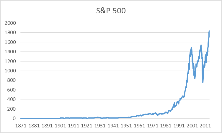
S&P 500 stock price index, 1871:M1 – 2014:M2. Data source: Robert Shiller.
On the other hand, if you plot these same data on a log scale, a vertical move of 0.01 corresponds to a 1% change at any point in the figure. Plotted this way, it’s clear that, in percentage terms, the recent volatility of stock prices is actually modest relative to what happened in the Great Depression in the 1930’s.
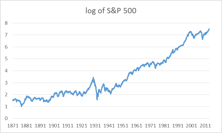
Natural log of U.S. stock prices.
There are a couple of other changes that can make the graph even more meaningful and easy to read. For one thing, we probably want to take out the effect of inflation. The graph below plots the natural log of the real instead of the nominal stock price, and subtracts off the log from 1871, so that the graph starts at zero and reports cumulative log returns since then. The numbers have also been multiplied by 100, so that if the value goes up by 1 unit on this graph, it corresponds to a 1% increase in the real value of stocks.
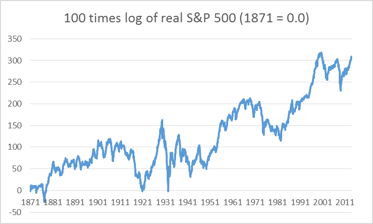
100 times difference between natural log of real stock price index at date t minus log of real stock price in 1871:M1.
Natural logs are also very convenient for describing relations between economic variables. For example, here’s a scatter plot of the relation between the log of U.S. real GDP on the horizontal axis (multiplied by 100 and normalized to begin at 0) and the log of U.S. oil consumption on the vertical axis. The relation between these series follows a straight line with slope of 1 up until about 1970, corresponding to an income elasticity of oil demand of around 1– for every 1% increase in real GDP, U.S. oil consumption also rose by 1%. By contrast, since 1970, the slope of the graph is about 0.2– U.S. real GDP has grown at a (continuously compounded) annual rate since then of 2.9%, whereas oil consumption has only grown 0.6%. You can read those numbers directly off the graph below by taking the difference between any two points and dividing by the number of years separating them.
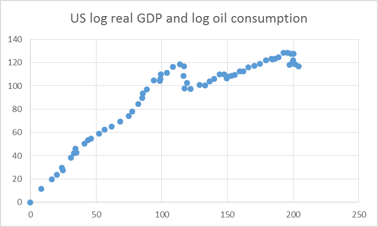
Horizontal axis: 100 times difference between natural log of real GDP in year t and value in 1949. Vertical axis: 100 times difference between natural log of U.S. oil consumption in year t and 1949. Data set covers 1949 through 2012.
So next time somebody wants to summarize data in terms of natural logs, don’t complain– it’s usually a much more meaningful and robust way to see what’s going on.
Very nice tutorial.
Bravo!
Now adjust the S&P 500 further for the US$ and GDP:
Not to mention that when you differentiate logs, you get the elasticity!
A graphical way of looking at this is that you want to show that percent difference is approximated by the log of their ratio:
In other words: (a – b)/b is approximated by ln(a/b)
The derivative of ln(x) = 1/x and is equal to 1 when x = 1
This means the tangent line to ln(x) when x = 1 is a line with a slope of 1 and y-intercept of -1, that is y = x – 1
Graphically the tangent line to ln(x) at x = 1 means that ln(x) is approximated by the line y = x – 1 when x is near 1
That is: ln(x) = x – 1 when x is near 1
Therefore: ln(a/b) = a/b – 1 = (a – b)/b when a/b is near 1
Lovely blog post.
I have had to learn to work with logarithms as part of my economics education but I had not (until now) realized just how helpful they can be.
More of this kind of thing, please. 😉
Let me agree with, Hugo. I encourage you to do teaching snipets like this one. Some of us took econ a long time ago, and a brief refresher on various topics is very welcome.
Professor Hamilton,
Regarding inflation, are you going to subtract an annual inflation percentage change from the log % change in the stock price or subtract a log percentage change in an inflation index or use some other calculation?
AS: First multiply the stock price at date t by the ratio of the CPI today to the CPI at date t. Then take logs. Equivalently you could first take the log of the nominal log stock price and subtract from it the log of the CPI as of that date. And here’s a third way (and how I in fact did it)– just download Shiller’s series for the real stock price from the source given.
Ah, all this is just talk. I’ll know you’re really committed to logs when we see them on the little math problems preceding the comments.
Thanks !
Just to point out if you don’t like e you can use any other base and get the same answers by dividing by the log to the new base of the old base. Other than because it appears in math formulas there is nothing really magic about e in a calculatory sense. I recall taking chemistry back before calculators when we had to use log tables to do problems because the answers needed 5 places of accuracy which a slide rule in general can not do. We used base 10 logs because the handbooks had more complete tables for them.
Logs are also useful when evaluating the forecast accuracy of an economic model. Many conventional measures of forecast accuracy such as signed mean percent error or MAPE are not symmetric. For example, a signed mean percent error calculation of (A-F)/A, where “A” is actual and “F” is forecast will limit the right tail to 1.00 as “F” approaches zero, but the left tail is unbounded. And this same asymmetry problem carries over to MAPE. But using the log of the ratio of forecast to actual (or vice versa, the absolute value is the same either way) will result in a symmetrical and unbounded histogram. Of course, the percent values have a different meaning, (e.g., 70% log error = 100% MAPE), but normally what you’re really interested in is the shape of the distribution and not the actual values along the horizontal axis of the histogram.
Professor Hamilton,
If I made the proper calculation, it seems that the rolling twelve month average return from 1871 to 2014 is about 2.1%. I seem to recall reading an article saying that investors are lucky to make 1% to 1.5% annual real returns after tax. I’d be interested in any comments you would like to make.
Have learned something from you, thx !
You seem to be a nice guy.
Keep on going – more interesting lessons for us, please! You know, we are all just an average joe, like Steven Kopits, Rick Stryker and me.
You could make something out of this blog putting it more to the broader community by being less sophisticated, presenting more general know-how.
Makes you more interesting !
Pls. tell this Menzie too.
Again, thanks a lot.
AS: The correct way to do this calculation is the simplest: take the log of the 2014 value minus the log of the 1871 value, and divide by the number of years, which is 0.0216, or a 2.16% average return. If you took the average of a rolling 12-month log difference, you would get almost the identical number (not quite identical, because the latter counts the years 1873-2012 more heavily than observations at the very beginning and end). But don’t forget the dividend return should be added to that 2.16% number.
Here’s another useful blog post on logs: http://blog.supplysideliberal.com/post/31224211784/the-logarithmic-harmony-of-percent-changes-and-growth
Professor Hamilton,
Thanks, I guess I was thinking about what an investor would expect for twelve month holding periods. I had made the 2.16 calculation to compute the average you mention, but was uncertain about what would be the best estimate of what an individual with a finite life could expect to earn per year (seems the difference is not material). Regarding the addition of the dividends from 1871 to 2013, I calculate about 3.56 as the average percent, if calculated correctly. Even with dividends included, it does not seem that the average investor in general makes an “unfair” amount (some seem to espouse) considering risk and taxes.
AS: You’d still want to do the calculation the way I described, even if your ultimate interest is to calculate the expected return over a typical 12-month holding period. If you go through the algebra, you’ll see that the only difference between the way I say the calculation should be done and the average using rolling windows of log returns is that the latter has a funny way of weighting the observations for 1871:M1 – 1871:M12 and 2013:M3 – 2014:M2 relative all the other observations in the sample. If you’re talking about a rolling window of percentage returns instead of a rolling window of log differences, that’s wrong for the same reason I explain in the text.
“So any time that you see a graph that is measured in logs, an increase of 0.01 on that scale corresponds very closely to a 1% increase.”
The problem I usually have with people using natural logs is that they don’t correctly reverse it (because they don’t understand whats going on and the effect of compounding). Like a blind rhesus money they do y=ln(P1/P0) in a spreadsheet and then L=(1+y)P0 to recalculate levels. For small numbers like 3-5% its not significant, but (as you know) the error grows with y or with the length of time. People with fancy MBA degrees. ugh. I had one student I tutored while he was getting his MBA (from a fancy school that shall not be named) tell me he had figured out a sure fire way to arb the market. haha. Every time I see a post like this, I think of that (and other) experiences and am reminded of Yoda’s wisdom: “First you must unlearn what you have learned.”
Don’t be so nasty to HBS !
Hi Mr. Hamilton,
could you please write a post about the 2008 fed transcripts, just like PK
did in
http://krugman.blogs.nytimes.com/2014/02/23/what-did-i-know-and-when-did-i-know-it-2
I am very sure the whole community would be interesting about your thinking !
Regards.