Among the disappointments in the 2015:Q1 GDP figures was weak consumption growth, which was a little surprising given the extra cash most consumers have on hand as a result of lower energy prices. I wanted to take a look at how the recent consumer behavior compares with what we’ve seen historically.
The graph below plots the price of energy goods and services relative to the overall price consumers pay for other purchases. Real energy prices have fallen about 20% from where they had been last summer.

Figure 1. Ratio of implicit price deflator for energy goods and services to overall PCE deflator, monthly 1959:M1 to 2015:M3.
Many consumers buy the same number of gallons of gasoline each week regardless of whether the price goes up or down. Such behavior would mean that someone who used to spend 5% of their budget on energy would only need to spend about 4% if energy prices fell 20%. And indeed we see in the data that purchases of energy goods and services now account for only 4.4% of total consumer spending, down from 5.6% a year ago.

Figure 2. Consumer purchases of energy goods and services as a percentage of total consumption spending, monthly 1959:M1 to 2015:M3.
In 2007, Paul Edelstein and Lutz Kilian studied the relation between energy prices and consumer spending using simple forecasting relations known as a vector autoregression. They summarized the effects on consumer budgets of energy prices by multiplying the monthly percent change in the relative price plotted in Figure 1 by the energy share in Figure 2– call this variable xt. Thus for example if the energy share is 5% and the price increases 20%, xt would equal 1, corresponding to the 1% loss of spending power described above. They then related xt to the monthly growth rate of real consumption spending. They used data from 1970:M7 to 2006:M7 to estimate a pair of forecasting equations to predict xt and real consumption growth based on observed values of the two variables over the previous 6 months. The black line in the graph below shows how an n-month ahead forecast of real consumption in that system would change when xt goes up by 1, a graph that economists describe as an “impulse-response function”. The green lines indicate 95% confidence intervals. Historically, an energy price increase that reduces consumer spending power by 1% would on average be followed within a few months by a 1% decline in real consumption spending and by closer to a 2% decline by the end of 6 months. One interpretation of why the latter effect is bigger than 1% is that it could reflect second-round macroeconomic multiplier effects of the lower consumer spending.
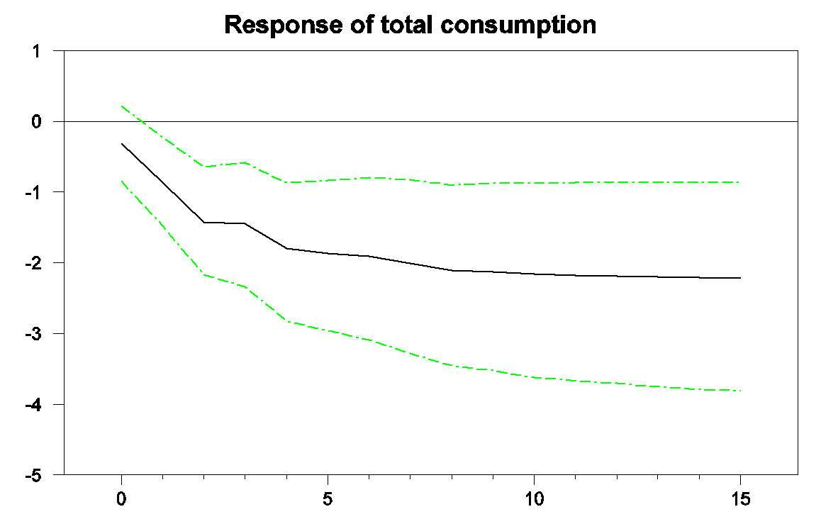
Horizontal axis: months after an increase in energy prices that would lower consumer spending power by 1% at time 0. Vertical axis: predicted percent change in real consumption spending between month 0 and month n. Source: based on Hamilton’s (2009) replication of Edelstein and Kilian (2007).
In a paper published in the Brookings Papers on Economic Activity in 2009, I looked at how much of the first-year’s downturn in consumption spending during the Great Recession could be accounted for by the sharp spike in energy prices that occurred at the time. The black line in the graph below plots real consumption spending between September 2006 and September 2008. It is measured as 100 times the natural log of real consumption, so that a one-unit increase on the vertical axis corresponds to about a 1% increase in real consumption spending. The trajectory of the black line shows the drop in consumption spending that preceded the Lehman bankruptcy in September of 2008.
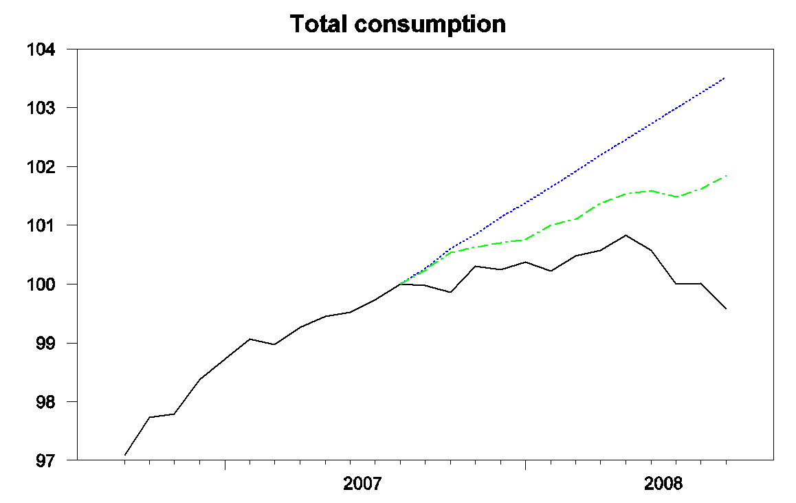
Black: 100 times the natural log of real consumption spending, 2006:M9 to 2008:M9, normalized at 100 for 2007:M9. Blue: forecast from the Edelstein and Kilian vector autoregression using only data as of 2007:M8. Green: forecast from the vector autoregression conditioning on observed energy prices over 2007:M9 to 2008:M8. Source: Hamilton (2009).
The blue line shows the predicted path for consumption based only on consumption and energy data available in September of 2007, while the green line shows the path predicted given the big increase in energy prices between September 2007 and July of 2008. The graph indicates that about half of the slowdown in consumption growth during the first three quarters of the Great Recession could be attributed to energy prices.
I was curious to update those calculations to take a look at the effects of the recent plunge in energy prices. I first re-estimated the Edelstein-Kilian vector autoregression using data from 1970:M7 through 2014:M7 and used the model to describe consumption spending since then. The black line in the graph below again shows the actual level of real consumption spending, this time for the period September 2013 through March of 2015. The blue line shows the forecast using data only available through July of 2014, before the big drop in energy prices. We would have predicted about a 2% increase in real consumption spending since July if there had been no drop in energy prices, compared with an actual increase in real consumption of 2.2%.
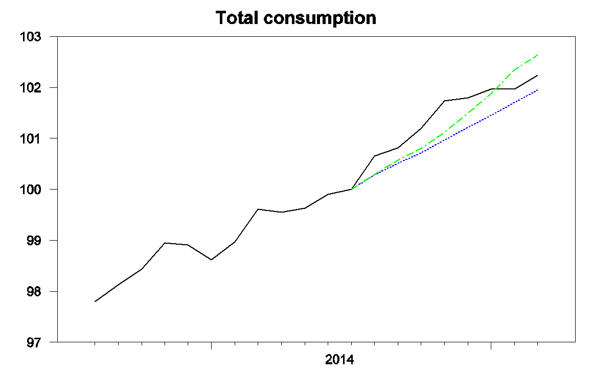
Black: 100 times the natural log of real consumption spending, 2013:M9 to 2015:M3, normalized at 100 for 2014:M7. Blue: forecast from an updated Edelstein and Kilian vector autoregression using only data as of 2014:M7. Green: forecast from the vector autoregression conditioning on observed energy prices over 2014:M8 to 2015:M3.
As before the green line indicates what we would have expected to see happen to consumption spending given the big drop in energy prices. Initially consumption was higher than predicted, with big gains in consumption spending coming before much of the decline in energy prices had actually reached consumers. But consumption since November has grown at a slower rate than would have been predicted even if there had been no drop in energy prices. Based on the historical relation between energy prices and consumer spending, we would have expected to see consumption today about 2.6% above where it had been in August rather than the observed 2.2% increase.
What’s different this time? Of course energy prices are just one of many factors influencing consumption spending and the differences highlighted above are modest. But the Wall Street Journal last week reported on a survey by credit-card issuer Visa that 70% of American consumers expect gasoline prices to go back up. This time consumers don’t trust the windfall to stay in their wallets, and so haven’t been spending the extra cash as freely as in the past.
Whatever the explanation, the facts seem to be that, unlike what we usually observed historically, consumers have been using much of the gains from lower energy prices to bolster their saving rather than using it to increase spending on other goods and services.
Take a look at “health” (a.k.a. as “illth”) care (HC)*** real spending per capita and as a share of real PCE per capita and its growth rate since 2000 and 2007 vs. gasoline and other energy’s share and rate.
http://research.stlouisfed.org/fred2/graph/fredgraph.png?g=1aT8
http://research.stlouisfed.org/fred2/graph/fredgraph.png?g=1aT9
http://research.stlouisfed.org/fred2/graph/fredgraph.png?g=1aTa
http://research.stlouisfed.org/fred2/graph/fredgraph.png?g=1aSV
http://research.stlouisfed.org/fred2/graph/fredgraph.png?g=1aSW
http://research.stlouisfed.org/fred2/graph/fredgraph.png?g=1aSX
http://research.stlouisfed.org/fred2/graph/fredgraph.png?g=1aSY
http://research.stlouisfed.org/fred2/graph/fredgraph.png?g=1aSZ
http://research.stlouisfed.org/fred2/graph/fredgraph.png?g=1aT0
Real growth per capita of HC spending is now accelerating to the rate at which recessions were underway in 2000 and 2007:
http://research.stlouisfed.org/fred2/graph/fredgraph.png?g=1aT2
http://research.stlouisfed.org/fred2/graph/fredgraph.png?g=1aT4
http://research.stlouisfed.org/fred2/graph/fredgraph.png?g=1aT5
Versus wages and salaries adjusted for core CPI:
http://research.stlouisfed.org/fred2/graph/fredgraph.png?g=1aTe
http://research.stlouisfed.org/fred2/graph/fredgraph.png?g=1aTf
http://research.stlouisfed.org/fred2/graph/fredgraph.png?g=1aTg
http://research.stlouisfed.org/fred2/graph/fredgraph.png?g=1aTh
Versus real final sales:
http://research.stlouisfed.org/fred2/graph/fredgraph.png?g=1aTm
http://research.stlouisfed.org/fred2/graph/fredgraph.png?g=1aTo
HC is a MUCH LARGER share of, and thus a drag on, real PCE, earned income, real final sales/GDP per capita than the household cost of energy.
With the US economy at or near the historical “stall speed”, accelerating growth of HC spending will constrain spending for other sectors indefinitely hereafter, all else equal.
The prohibitive, increasingly financialized (via insurance) cost of HC is contributing incrementally to falling labor’s share and the decelerating growth of real productivity, private investment, wages, and capital formation. Gov’t-sponsored, enabled, and protected for-profit “illth” care is killing the economy. “The market” for HC profits will only continue to “succeed” in encouraging the same incentives and net flows that have gotten us where we are today. A single-payer system, sizable incentives for lifestyle improvements, and rationing of appallingly costly late-life procedures, treatments, and medications are the only long-term solutions to REDUCING “illth” care spending to wages, PCE, and GDP.
Of course, there is no political constituency to challenge the insurers, hospital companies, pharma, biomedical, and the AMA, the principal interests who disproportionately benefit from the prohibitively costly for-profit system that the country cannot afford.
***http://www.nihcm.org/pdf/DataBrief3%20Final.pdf: 50-65% to 80% of HC spending (~18-19% of GDP, $10,000 per capita, 42% of wages and salaries, and $26,000 per household) is on the sickest 5-10% to 20%. The lower 50% of households account for 3% of spending. 15% of household spend nothing on HC. 20% of HC spending is on costly procedures and treatments for elders in late life or at end of life. This is ABSOLUTELY APPALLING and will likely be a further incremental drag on PCE and the economy overall as peak Boomers age into end of life and draw down en masse on Medicare and Medicaid. HC is no longer a net value-added service but a net cost to the US economy and society.
most people who buy gasoline put it on their credit card, and there were corresponding decreases in credit card balances in January and February before they rose in March…i’d suggest most of us dont see lower gas prices as “having more money to spend”
If gasoline prices are such a windfall and consumer spending is down, what’s this all about? http://www.federalreserve.gov/releases/g19/current/
@Bruce Hall:
Real per capita consumer credit less student loans:
http://research.stlouisfed.org/fred2/graph/fredgraph.png?g=1aUU
Less student loans and auto loans:
http://research.stlouisfed.org/fred2/graph/fredgraph.png?g=1aUV
Auto loans:
http://research.stlouisfed.org/fred2/graph/fredgraph.png?g=1aV3
http://research.stlouisfed.org/fred2/graph/fredgraph.png?g=1aV2
Subprime auto loans:
http://www.nytimes.com/2015/03/02/business/dealbook/wells-fargo-puts-a-ceiling-on-subprime-auto-loans.html?_r=0
http://fortune.com/2015/01/13/subprime-auto-loans/
” This is ABSOLUTELY APPALLING and will likely be a further incremental drag on PCE and the economy overall as peak Boomers age into end of life and draw down en masse on Medicare and Medicaid. HC is no longer a net value-added service but a net cost to the US economy and society.”
And single payer fixes this how?
Yes, the permanent income hypothesis is the orthodox explanation.
Steven Kopits’ outlook for global total liquids supply less demand, prepared in January, 2015 (Steven’s outlook is Preinga):
http://i1095.photobucket.com/albums/i475/westexas/Supply%20Minus%20Demand_zpswyvmrvkw.png
The (so far) monthly low Brent for the current oil price decline was January, when Brent averaged $48. Assuming that Brent averages about $65 for May, the annualized rate of increase in monthly Brent crude oil prices from 1/15 to 5/15 will have been about 90%/year, which would seem to be consistent with Steven’s forecast.
Note that the annualized rate of increase in monthly Brent crude oil prices from 12/08 (the low point for the previous large oil price decline) to 2/15 was 43%/year.
In other words, monthly Brent oil prices are currently recovering at about twice the rate that we saw from the 12/08 low to 2/11, when Brent once again averaged $100.
However, one quibble that I have with the global liquids analysis is that it does not take into account generally rising consumption in oil exporting countries, i.e., global total liquids supply can increase, but the volume of net exports available to importers can fall, which is what we have seen since 2005.
The volume of what I define as Global Net Exports of oil (GNE*) fell from 46 MMBPD (million barrels per day) in 2005 to 43 MMBPD in 2013 (2014 data not year available), as annual Brent crude oil prices doubled from $55 in 2005 to an average of $110 for 2011 to 2013.
The volume of GNE available to importers other than China & India fell from 41 MMBPD in 2005 to 34 MMBPD in 2013, while the US remains reliant on net crude oil imports for about 44% of the crude + condensate processed daily in US refineries.
At the 2005 to 2013 rate of decline in the ratio of GNE to Chindia’s Net Imports (CNI), the volume of GNE available to importers other than China & India (Available Net Exports, or ANE) would theoretically approach zero in about 17 years. Note that Chinese oil imports reportedly hit an all time record high in April, 2015. Historical and projected Chinese car sales:
http://i1095.photobucket.com/albums/i475/westexas/Chinese%20Vehicle%20Sales_zpsthm0iaxa.gif
Given an ongoing (and inevitable) decline in GNE, it’s a mathematical certainty that unless CNI falls at the same rate as the rate of decline in GNE, or at a faster rate, the rate of decline in ANE will exceed the rate of decline in GNE, and the rate of decline in ANE will accelerate with time.
For more info, you can search for: Export Capacity Index.
*Combined net exports from (2005) Top 33 net oil exporters, total petroleum liquids + other liquids, EIA data
Typo correction:
Note that the annualized rate of increase in monthly Brent crude oil prices from 12/08 (the low point for the previous large oil price decline) to 2/11 was 43%/year.
There is also a component of inflation expectations. There is no need to spend money if it is not going to lose value over time. You can save for large purchases without having to building in some kind of hedge. When consumers expect their dollars to depreciate they will buy products that they may not need immediately to anticipate price increases.
Surprisingly, we can thank Janet Yellen for much of this. She has actually done a decent job of managing the purchasing power of the dollar. She is certainly not Paul Krugman.
Permanent income hypothesis
Gonna be fun to watch Q2 PCE spending accelerate rapidly. You guys have to get off 1 quarter confirmation biases.
@Rage, notwithstanding what will be reported tomorrow for retail sales, various private surveys for retail sales suggest that sales growth has decelerated during the first six weeks of Q2, averaging ~1.7% YoY, with the YTD YoY rate slightly below the 3% YoY trend for the past couple of years.
That translates to a nominal GDP YoY of just ~2.4% (vs. 3.4-4.5% in 2014) for Q2 and real SAAR GDP for Q2 of a bit less than 1%. At the trend rate of the deflator, real GDP YoY and the 4-qtr. average through Q2 suggests real GDP decelerating to the historical “stall speed” of ~2%.
Moreover, given the retail sales surveys, implied nominal and real GDP, and US Treasury withholding receipts, employment is likely to be overstated, growing little, if at all, YoY.
Given the surge in health care spending and as a share of GDP and PCE, a sustained increase in the price of gasoline will be a marginal constraint on the growth of spending that is already decelerating, especially for the bottom 90%+ of households.
Finally, with the jump in inventories in Q1 (assuming it holds) and the YoY contraction of orders, I suspect that industrial production mfg. is set to decelerate more than is generally expected, reinforcing the slowdown in spending and affirming the suspicion that employment is overstated since the peak in Aug-Nov 2014.
Why do you assume “extra cash”? The more likely situation is paying off debt and/or not going further into debt, e.g., when their credit card is maxed out or they can’t get new credit.
“Many consumers buy the same number of gallons of gasoline each week regardless of whether the price goes up or down.” What, if any, is the proof of this statement from the article? I know for many their lifestyle makes it difficult for them to reduce fuel consumption below some minimum threshold but I’m pretty sure all but the most well off found some way to do so.
Again these short-term seadonally adjusted numbers are too uncertain to be worth this much analysis. You’re really just guessing that savings increased; it could also be that real income growth failed to accelerate due to weakness elsewhere, or that consumption has accelerated more than our measuring methods have captured.
The perfect time to institute Pigou taxes on oil consumption.
Agreed. Reduce carbon and particulate emissions. Drive US energy intensity to the point that energy shocks no longer threaten macroeconomic stability.
The definitive refutation of the so-called “shale revolution”:
http://www.artberman.com/wp-content/uploads/DGS-Presentation-12-May-2015_Reduced.pdf
The critical issue of “exergy” and the prohibitive energy cost of energy extraction of costlier, lower-quality crude oil substitutes:
http://www.thehillsgroup.org/
Peak Oil is in the rear view mirror. The global structural constraints to growth of real GDP per capita from Peak Oil, the log limit bound of systemic exergy, and rate of growth of net energy flows/throughput per capita will persist indefinitely hereafter, reflecting “Limits to Growth” and eventual peak and decline of population at some point in the decades ahead.
Without growth of profitable extraction of crude oil substitutes, production and consumption will continue to decline per capita, real GDP per capita will continue to decelerate, and we will not be able to afford to sustain the build out of renewables AND maintain the existing fossil fuel infrastructure AND replenish the deteriorating, complex, high-tech, high-entropy national infrastructure.
Good piece.
See? Even consumers did not expect oil prices this low. Everybody and I mean everybody got oil price forecasts wrong.