There was lots of action in financial markets last week, with much of the attention focused on the U.S. Federal Reserve. The interest rate on a 10-year U.S. Treasury bond edged up 10 basis points early in the week in anticipation that the Fed might finally raise its target for the short-term interest rate. But it shed all that and more after the Fed announced it was standing pat for now.
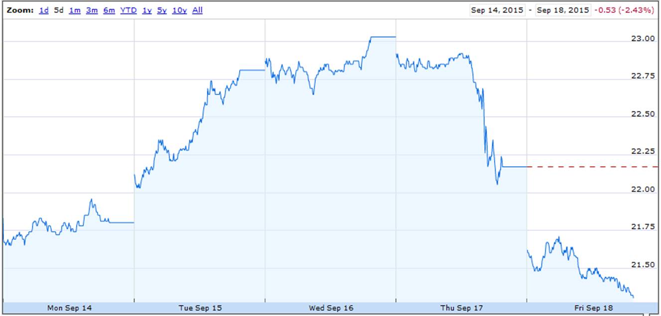
Price of CBOE option based on 10-year U.S. Treasury yield; to convert to the Treasury yield itself divide by 10. Source: Google Finance.
If bond investors were rational and unconcerned with risk, the 10-year rate should correspond to a rational expectation of what the average short-term rate is going to be over the next decade, a conjecture known as the expectations hypothesis of the term structure of interest rates. If instead the 10-year rate was above the average of expected future short rates, you’d expect a higher return from the long-term bond than staying short. If you were risk neutral, you’d prefer to go long in such a setting. But if more investors tried to do that, it would drive the long yield down and the short yield up.
If the expectations hypothesis held true, it’s hard to see how swings of the magnitude observed this week could be driven by news about the Fed. Although the Fed did not raise the overnight rate this time, it probably will by the end of this year or early next. A difference of 50 basis points for 1/4 of a year amounts to a difference of (1/40)(50) = 1.25 basis points in a 10-year average, only a tenth the size of the observed movement. Maybe people see the Fed’s decision as signaling a change in the interest rate that it will set over a much longer period, not just 2015:Q4. Or perhaps the nature of this week’s news altered investors’ tolerance for risk. To the extent that the answer is the latter, can we describe empirically the forces that seem to be driving the changes in risk tolerance and quantify the magnitude of the changes over time?
The nice thing about questions like these (unlike many of the other thorny unsettled issues in economics) is that in principle they could be resolved by an objective analysis of the data. All we need is to calculate the rational forecast of future interest rates, and compare those forecasts with the observed changes in long versus short yields.
The first step in this process is to determine the variables that should go into these forecasts. Finding the answer to this question is the topic of a paper that I’ve recently finished with Michael Bauer. Michael is an economist at the Federal Reserve Bank of San Francisco, though I should emphasize that the views expressed in the paper are purely the personal conclusions of Michael and me and do not necessarily represent those of others in the Federal Reserve System. Our paper confirms the finding from a large earlier literature that the expectations hypothesis cannot fit the data, adding lots of new evidence of predictable changes in long rates that cannot be accounted for by a rational expectation of future short rates. But we disagree with the conclusion from a number of recent studies that claim that all kinds of variables may be helpful for predicting interest rates.
We investigate instead a less restrictive model than the expectations hypothesis, which we refer to as the “spanning hypothesis,” that posits that whatever beliefs or risks bond prices may be responding to, these are priced in a consistent way across different bonds with the result that you only need to look at a few summary measures from the yield curve itself to form a rational forecast of any interest rate at any horizon. We calculate these summary measures from the first three principal components of the current set of yields on all the different maturities. Though the principal components are calculated mechanically, they have a simple intuitive interpretation. The first is basically an average of the current interest rate on bonds of all the different maturities (referred to as the “level” of interest rates), the second measures the difference between the yield on long-term bonds and short-term bonds (a.k.a. the “slope” of the yield curve), and the third reflects how much steeper the yield curve is at the short end relative to the long end (the “curvature” of the yield curve).
The main contribution of our paper is to show why other researchers were misled into thinking variables besides these three factors might help predict interest rates. It’s long been known that one has to be careful using regression t-statistics to interpret the validity of predictive relations when the explanatory variables are highly persistent and correlated with lagged values of the variable you’re trying to predict, a phenomenon sometimes described as Stambaugh bias; Campbell and Yogo have a thorough investigation of this phenomenon. My new paper with Michael identifies a different setting in which a related problem can arise. Namely, if you add other extraneous highly persistent regressors to a regression for which the coefficients on the true predictors would be susceptible to Stambaugh bias, any of the usual procedures for estimating the standard errors on those extraneous variables, such as heteroskedasticity- and autocorrelation-consistent standard errors, will significantly overstate how precisely you have estimated the coefficients, even if the extraneous predictors have nothing at all to do with either the true predictors or the variable you’re trying to predict. In our setting, the variable we’re trying to predict is the excess return on a particular bond, and what we claim are the true predictors are the level and slope of the yield curve (both highly persistent and correlated with lagged values of excess returns). That means when you add another variable to the regression that’s highly persistent such as inflation or measures of GDP, you’ll think you have something statistically significant when it fact it is of no use at all in predicting interest rates.
In addition to working out the econometric theory for how this happens, we develop an easy-to-implement bootstrap representation of the data in which the only variables that can predict interest rates or bond returns are the level, slope, and curvature, and investigate what would happen in such a setting if you performed the kinds of analyses conducted by earlier researchers. We find that a researcher could easily mistakenly think he or she had found a useful predictive relationship when the reality is that there is none, and show point by point how the findings of previous studies are completely in line with the claim that only three variables are of any use for predicting interest rates. We also find that an ingenious test proposed by Ibragimov and Mueller can sometimes work very well to detect the problems in this setting. Basically their test tries to estimate the standard error of coefficients by seeing how much they differ when estimated across different samples. Here again one finds a warning flag in the earlier studies– the apparent predictability of interest rates seems very strong for a short time, but then falls apart on other data.
Our study also updates many of the models estimated by previous researchers, and finds that none of these proposed forecasting relations has held up very well in the data that came in after the original study was first published. By contrast, the predictive power of the level and slope hold up quite well in any subsample we looked at, confirming the solid rejection of the expectations hypothesis in the earlier literature.
The bottom line: bond returns and departures from the expectations hypothesis are predictable. And it’s easier to do than some studies have been suggesting.
Here’s the summary from the paper:
A consensus has recently emerged that a number of variables in addition to the level, slope, and curvature of the term structure
can help predict interest rates and excess bond returns. We demonstrate that the statistical tests that have been used to support this conclusion are subject to very large size distortions from a previously unrecognized problem arising from highly persistent regressors and correlation between the true predictors and lags of the dependent variable. We revisit the evidence using tests that are robust to this problem and conclude that the current consensus is wrong. Only the level and the slope of the yield curve are robust predictors of excess bond returns, and there is no robust and convincing evidence for unspanned macro risk.
All bonds means all safe bonds? Is there a risk term for private bonds following the same rule or a similar rule with different parameters?
Lord: Sorry, I should have clarified that we’re just talking about Treasuries.
A short-term explanation may be the Fed signaled to financial markets, changing some beliefs, the economy is weaker than reflected in the data, and there’s an expectation bonds will outperform stocks.
Of course, longer term, the bond market doesn’t expect short-term interest rates to rise much.
Econometrics aside…one can only ask… Who cares?
The shape of the yield curve whether 3 factors or five… is merely seen as the raw input necessary to “calculate” the forward rates.
In an efficient market, technicians will calculate the “effective cost of creating these forwards”… taking into account the usual arbitrage
constraints.
In the past 10 years or so, this function has been subsumed by the marketplace in both mid curve “Eurodollar futures” and more importantly,
the complete array of options on these deferred forwards. (Thes forwards and their options extend now to 2020 (the purples). These contracts, particularly the December “series” are known as surrogates for the FED’s SEP “dots”… extending all the way out to 2020. Its as though the HJM world has been created just for speculators. The simultaneous development of the forward FRA/OIS marketplace has tied these deferred Eurodollar contracts directly to OIS.
I’ve enclosed the path of the DEC 2018 market “Dot”…since the beginning of this year. the EDZ 2018 Eurodollar transformed into One Month OIS… commonly know as “The Terminal Rate”. Over the course of this year… that “Terminal Rate” expectation has had more than a 300 basis point range… indeed since the June FOMC its dropped nearly 70 basis points.
While you note that “A difference of 50 basis points for 1/4 of a year amounts to a difference of (1/40)(50) = 1.25 basis points in a 10-year average, only a tenth the size of the observed movement. ” if every 1/4 of a year rate moves up 50 basis points or down … and the Ten year note is nothing but the average of 40 such rates…. why should one be surprised if the average itself moves substantially,
Stan Jonas
https://onedrive.live.com/redir?resid=30E4BD8F5396E356!9054&authkey=!AANaC9tmuPa-4Jw&v=3&ithint=photo%2cpng
Stan Jonas: Yes, the forward curve is just an equivalent way of summarizing exactly the same numbers as in the yield curve. But no, the forward curve is not the optimal forecast of future short rates. It would be the optimal forecast only if the expectations hypothesis were true.
As for your point about the 10-year yield, yes, if this means a change in future short rates and not just for 2015:Q4 it could mean a bigger change in the long yield. That’s exactly what I said. But I don’t see why it does signal a change in the rate for 2016:Q1 or any quarter thereafter. I thought that 2016:Q1 will be 50 bp before the FOMC meeting, and I still think that 2016:Q1 will be 50 bp after the meeting.
A smart, solid critique. Well done.
I’m confused though by this statement: “it is not necessary to look beyond the information in the yield curve to estimate risk premia in bond markets.” It seems to me the yield curve always combines future expectations for short rates with risk premia and does not distinguish between them. Perhaps I’m misunderstanding what you’re trying to say.
Also you leave the reader hanging with this question: “To what extent does this represent unprecedentedly low expected interest rates extending through the next decade, and to what extent does it reflect an unusually low risk premium resulting from a flight to safety and large-scale asset purchases by central banks that depressed the long-term yield?”
My feeling is that the jury is out on whether changing the composition of public liabilities from longer-term to shorter-term through LSAP really depresses the risk premia on longer-term public liabilities. It’s definitely not as simple as less supply of x means higher price of x. These are financial assets not real goods. The pool of savings vehicles is big and diverse, and savers can adjust in various ways. Moreover one element of risk premia is liquidity risk.
Tom Warner: We’re saying that both expectations and risk premia are embodied in current yield curve. You can read both off of current yields alone. But as I explained to Stan Jonas above, you don’t do it with forward rates. We infer the risk premia by estimating the rational forecast of future rates and then calculating the difference between that and the forward rate.
So what will the US 10-year Treasury note yield be in December 2016?
JBH: I don’t know, and don’t claim to know. I use “optimal forecast” in the sense of having the forecast with a lower mean squared error than any other forecast. That is not the same thing as having a forecast whose mean squared error is zero.
JDH: Thanks for responding. Your paper claims to have improved on the consensus models used to predict interest rates. My question, as I hope you might have gathered, was getting at a deeper thing than a mere point forecast. It was taking the claim you make in your paper and asking for a forecast of the future. The only true test of how your model works must come in real time. I for one don’t buy the result of your paper, which I take to be that nothing other than the level, slope, and curvature of the yield curve have ever been shown to predict interest rates with greater accuracy than these. Said another way, all can be subsumed into interest rates so that when all is said and done only interest rates predict interest rates.
Now ask yourself. In the real world, are there not a myriad of factors that affect interest rates? Of course. One sees this daily in the way the market moves. To not burrow deeper is to halt science. Would Richard Feynman have stopped there? I pick Feynman because to me he most epitomizes the scientist who more than anything wanted to get to the bottom of whatever it was that struck his curiosity.
Interest rates possess a curious trait. On the margin, they are driven in actual real world cause and effect fashion by a plethora of forces. Some of these are veritable constants. Inflation, for example. And I have no doubt that variables of this class can be codified for the most part in the yield curve and its shape. This is, to me, basic stuff. But it is that other class of variables – those that come and go and come back, and those that come and go never to be seen again – that are what science needs to plumb. An example is the euro crisis in 2011. A never-before-seen event on a scale like this that dramatically affected US yields via flight to safety.
Hence if I may state boldly, the consensus framework, on which this paper is a tiny tweak, needs to be jettisoned. Keeping, of course, the robust timeless part. To truly advance the science of interest rate projection, an entire new mathematics needs to be created. I am not sure that the mathematics I envision is possible. But deep down I suspect it is. It would be as revolutionary as the invention of the calculus. In place of that and until then, scientists will have to settle for second best.
Second best is recognizing the aforementioned curious trait and incorporating it in serious research. Event analysis is perhaps the methodology closest to the way the field has to go. For interest rates are hugely context sensitive. The context of the historic moment matters, and it matters greatly. Some new event enters the picture. The market recognizes it, acts on it, and for a time is both carried by and sometimes carried away by it. China, for example, played a big role in the Greenspan conundrum in 2004. There may have been something like China and a Greenspan-type conundrum in the distant past. But not in modern times. So with no prior observations on this new variable, regression analysis would have been of little help in forecasting interest rates in real time.
As any new force like this robustly affects interest rates at the margin, but by definition does not do so in prior quarters and years by dint of being new, regression analysis does not and cannot pick up on it. Regression analysis simply homogenizes the multiple brilliant shades of the real world into a dull brown. For regression does not, nor can it, recognize the context surrounding each of the n observations that go into calculating the relative handful of estimated coefficients. You may well understand this. Others may have to think about this some. But reliance on a methodology that takes the marginality of the universe and averages it into a handful of coefficients is precisely why the consensus has not gotten very far in predictive accuracy.
My above question about where does your model predict interest rates will be a year from now was to get at this by exposing the truth content of the model. I already know the answer in a probabilistic sense by dint of years of study and expertise gained in forecasting rates. I will bet that the model’s future forecast – the only kind of forecast that matters since it is truely out of sample – will be in significant error.
The WSJ consensus projects the 10-year will be 3.09% in December 2016. It is only natural for those of us who frequent this site to want to know what a model purporting to be more optimal than the consensus might say. A point estimate would be a start, though a band around it would certainly be acceptable as well.
Question: as I understand the Fed these days, it can’t just raise the “Federal funds rate” like it used to because the reserve system is wallowing in reserves (and because non-bank financial institutions also have excess cash), so they are planning on increasing the amount of interest they pay on reserves to make it unattractive to lend for less AND they’re planning on buying lots of cash from non-bank institutions so they’ll also be making more interest on enough cash that lending for less is unattractive. I gather they’ll still talk about the interest rate range but may actually raise the interest they pay to as much as 1%. If so, how can that be effectively modeled other than as a guess until it happens (and is effective or not)?
jonathan: The FOMC has formulated the principles and mechanics for managing short-term interest rates when these will be raised, a process which it refers to as “policy normalization.” These can be found here. In addition, the Fed has recently released a useful primer on its changing approach to policy implementation. As you correctly note, part of this will be an increase in the IOER rate, but there are also other tools to maintain an effective corridor for short rates, such as overnight reverse repos.
How does this relate to our paper? Our focus is on forecasting the overall level of yields as well as bond returns, which are determined by long-term interest rates. The institutional details at the short end of the yield curve have only limited importance for this. They simply constitute an additional source of uncertainty which makes it harder to predict the future (until it becomes clearer what policy normalization exactly looks like). Our point is that what we can predict for the future of interest rates, we can learn by just observing the current yield curve, and we do not need to incorporate additional information from macro variables, surveys, or other sources.
This is very interesting work! I was wondering about the connection to pseudo-out-of-sample evaluations: if these authors who claimed to find all these unspanned factors had performed out-of-sample evaluations, they would have found that their factors actually do not help, right? Put differently, would a simple pseudo-out-of-sample evaluation be a third method besides the two tests that you suggest or are your tests in some way related to a out-of-sample evaluation or are your tests and pseudo-out-of-sample evaluations somehow related anyways?
Chris: Yes, the Ibragimov-Mueller test can be thought of as a version of testing for out-of-sample forecast performance. But whereas most standard tests of the latter just arbitrarily divide the sample into separate estimation and evaluation subsamples, the IM test makes use of the complete sample of data for both tasks.
Professor Hamilton,
Would you suggest a beginning to intermediate source for readers to understand the relationship between short-term and long-term rates with the aim to allow such readers to have a sense of how this knowledge leads to the forecast of long-rates given short-rates?
AS: You might take a look at Chapter 10 in “The Econometrics of Financial Markets” by Campbell, Lo, and MacKinlay.
Thanks!
I purchased “The Econometrics of Financial Markets”. Chapter 10 is a challenge as I am sure the entire book will be. I am familiar with present value calculations. The authors’ extra subscripts used for precision sometimes can seem confusing. I could not find a “student” website that I find useful for my accounting students for the various assigned accounting texts. I did need to review several other sources in order to calculate forward rates. I wish that the authors’ showed more numerical examples in order to fix their concepts in the reader’s mind.
Any chance you would consider updating your post on forward rates from November 24, 2013? I would like to see some numbers used in equation (21) from the Gurkaynak, Sack & Wright paper. I downloaded the data file and see the various beta and tau coefficients that are updated as of 9/23/2015. My calculations of the forward rates for the 1,4 and 9 year periods seem to be off by a bit.
Being in the category of general audience reader, I am not able to decipher how to convert the formidable work presented in your paper into a forecasting model (my ignorance). Is it possible to present a regression model that a general reader could use to attempt a forecast of interest rates? Does it make any sense to compare the forecasts from your paper with the forecasts presented in the November 24, 2013 blog?
I believe there is logical issue. The 10 year yield is not the same as the ten year zero-coupon rate. But you seem to be suggesting that it is the same, thus getting the conclusion that the 10 year yield is the (geometric) average of (1+ ) short term rates (- 1). This is true for the 10 year zero, not the 10 year bond yield.
Pete: That’s a valid point. Our empirical work is based on the prices of zero-coupon bonds. But for purposes of this blog post I was trying to explain what the research means in terms that a general audience could follow.
I have an easier method.
Q: Is Govt Debt / GDP high?
If yes, rates will remain low.
Since Govt Debt / GDP will remain high and likely going higher, and exploding again during the next recession, rates will remain low because the US Govt can’t afford higher rates on Govt debt without crowding out entitlements and the military. And the Fed isn’t independent. They are enablers to the alcoholic govt.