How can we estimate the separate economic effects of shocks to oil supply and demand? I’ve just finished a research paper with Notre Dame Professor Christiane Baumeister that develops a new approach to this question.
The basic reason the question is hard to answer is that we would need to know the value of two key parameters: the response to price of the quantity supplied (summarized by the supply elasticity) and the response to price of the quantity demanded (summarized by the demand elasticity). If we only observe one number from the data (the correlation between price and quantity), we can’t estimate both parameters, and can’t say how much of observed movements come from supply shocks and how much from demand.
One way to resolve this problem is to find another observed variable that affects supply but not demand. A generalization of this idea is the basic principle behind what is referred to as structural vector autoregressions, in which we might also exploit information about the timing of different responses. The simplest version of this would be an assumption that it takes longer than one month for supply to respond to changes in price. If the very short-run supply elasticity is zero, and if supply shocks are uncorrelated with demand shocks, then the correlation between the error we’d make in forecasting quantity and price one month ahead could be interpreted as resulting from the very short-run response of demand to price. Putting this together with the observed dynamic correlations between the variables (for example, the correlation between this month’s quantity and last month’s price) would allow us to identify the effects of the different shocks over time.
In a previous paper that will be published in the September issue of Econometrica, Christiane and I proposed that Bayesian methods could allow us to generalize the traditional approach to structural vector autoregressions. We noted that what is usually treated as an identifying assumption (for example, the restriction that there is zero response of supply to the unexpected component of this month’s change in price) could more generally be represented as a Bayesian prior belief– we may believe it’s unlikely there is a big immediate response of supply to price but should not rule the possibility out altogether. Our paper showed how one can perform Bayesian inference in general vector dynamic systems where there may be good prior information about some of the relations but much weaker information about others.
In our new paper Christiane and I apply this method to study the role of shocks to oil supply and demand. We begin by reproducing an influential investigation of this question by University of Michigan Professor Lutz Kilian that was published in American Economic Review in 2009. Kilian studied a 3-variable system based on oil production, price and a measure of global economic activity. He assumed that supply does not respond contemporaneously to price or economic activity and that economic activity does not respond contemporaneously to oil production, assumptions that are referred to as the Cholesky approach to identification.
We first reproduced Kilian’s results using his dataset and his methodology. The panels below summarize the effects of three different kind of shocks (represented by different rows) on each of the three variables (represented by different columns). The horizontal axis in each panel is the number of months since the shock first hits at date 0. The red lines are the estimates that Kilian came up with based on his Cholesky identification.
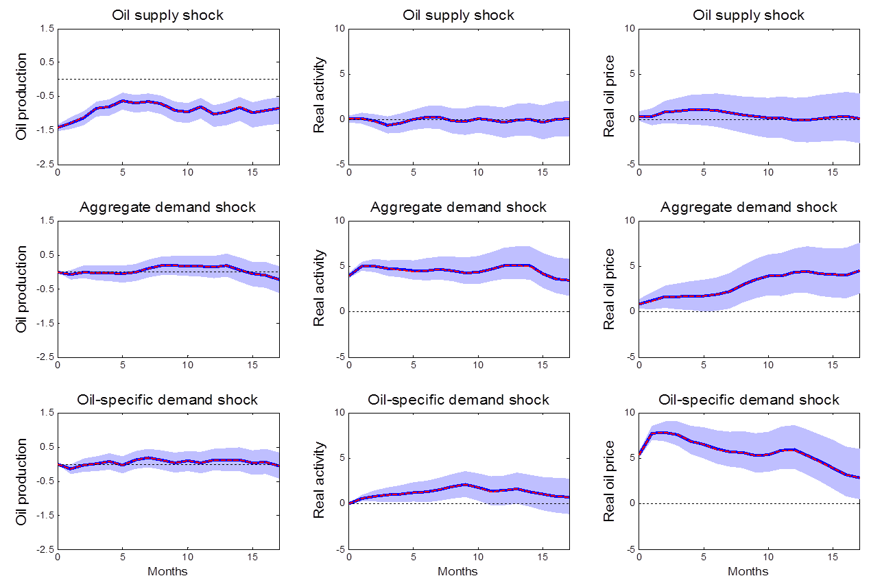
Effects of 3 different shocks on 3 different variables as estimated using the Kilian (2009) Cholesky identification. Red lines give Kilian’s original estimates. Blue lines and shaded regions give posterior medians and 95% posterior credibility sets when the approach is implemented as a special case of Bayesian inference. Source: Baumeister and Hamilton (2015).
We then formulated the same approach as a special case of Bayesian inference, in which we have dogmatic prior beliefs about the contemporaneous response of supply to price and economic activity but very uninformative prior information about the contemporaneous response of demand to price and economic activity. We conducted this Bayesian inference as a special case of the algorithms developed in our Econometrica paper. Incidentally, anybody can download the MATLAB code to do this kind of exercise themselves from my webpage. The Bayesian posterior median and 95% posterior credibility sets are indicated in blue. Not surprisingly, these are exactly the same answer as Kilian obtained using the traditional method.
Is there any benefit to reframing the traditional approach as a special case of Bayesian inference? One of the natural byproducts of our algorithm is the Bayesian posterior inference (that is, what we believe now that we have seen the data) about magnitudes such as the short-run demand elasticity of oil. It turns out that if we had the Bayesian prior beliefs that are implicit in Kilian’s approach, now that we have seen the data, we would still insist that the short-run supply response is zero (because our Bayesian prior beliefs about this parameter were dogmatic), but we would now also be very confident that the short-run demand elasticity is greater than two in absolute value and readily believe that it might be minus or plus infinity. In other words, we do not regard it as the least implausible to conclude that within a month of a 1% increase in oil price, in response consumers might increase their consumption of oil by a million percent or more. Quoting from our paper:
The claim that we know for certain that supply has no response to price at all within a month, and yet have no reason to doubt that the response of demand could easily be plus or minus infinity is hardly the place we would have started if we had catalogued from first principles what we expected to find and how surprised we would be at various outcomes. The only reason that thousands of previous researchers have done exactly this kind of thing is that the traditional approach required us to choose some parameters whose values we pretend to know for certain while acting as if we know nothing at all about plausible values for others. Scholars have unfortunately been trained to believe that such a dichotomization is the only way that one could approach these matters scientifically.
Misgivings about the traditional method are one reason that many researchers have looked for other approaches to identification, such as relying on sign restrictions– surely we can at least rule out that consumers increase the quantity they buy when the price goes up. In a subsequent paper with University of Virginia Professor Daniel Murphy, Kilian used sign restrictions to achieve partial identification and replaced the assumption that there is no contemporaneous response of supply with a hard upper bound on the size of the contemporaneous response. My paper with Christiane shows that the Kilian-Murphy results can also be obtained as a special case of Bayesian inference. We note among other concerns that their specification still allows for an implausibly large contemporaneous response of demand, ignores a good deal of other informative prior information, and yet is still dogmatic about other magnitudes that we really do not know for certain.
The main point of our paper is that if researchers had thought about what they were doing as a Bayesian exercise from the very beginning, there is a much richer set of prior information that could be drawn on while simultaneously relaxing many of the dogmatic restrictions. We illustrate how this can be done for the question of the role of oil supply and demand shocks in particular. Among other contributions, as in a later paper by Kilian and Murphy (2014) we bring inventories into the analysis (as a key reason why quantity and price need not move together), allow for measurement error in the variables (a ubiquitous problem in macroeconomics that is usually entirely ignored in most research), allow the possibility that the relations have changed over time (with the Bayesian approach offering a middle ground between assuming on the one hand that all the data are equally useful or throwing out earlier data altogether on the other), and make use of detailed evidence from other datasets about the price and income elasticities of supply and demand.
The figure below presents a few of the results we come up with. These are dynamic responses (like those in the first figure above) of global industrial production (the first column) and the real oil price (the second column) to each of the four shocks we study (shocks to supply, economic activity, oil consumption demand, and inventory demand). All four shocks would raise the price of oil, as seen in the second column. But whereas an oil price increase that results from a supply reduction leads to a decline in economic activity, the same is not true of an oil price increase that results from an increase in demand.
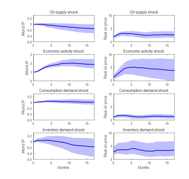
Effects of 4 different shocks on 2 different variables as estimated using the general Bayesian approach in Baumeister and Hamilton (2015). Blue lines and shaded regions represent posterior medians and 95% posterior credibility sets.
Another thing we do in the paper is look at the contribution of different shocks to historical movements in each of the variables. The red lines in each of the 4 panels below plot the actual percent change in the crude oil price each month over 1975-2014. The blue lines give the Bayesian posterior estimate of how big the percent change that month would have been if there had been only one shock. For example, the first panel isolates the contribution of supply shocks. Ninety-five percent posterior credibility regions for the estimates are indicated by light blue shaded regions.
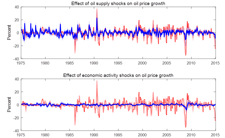
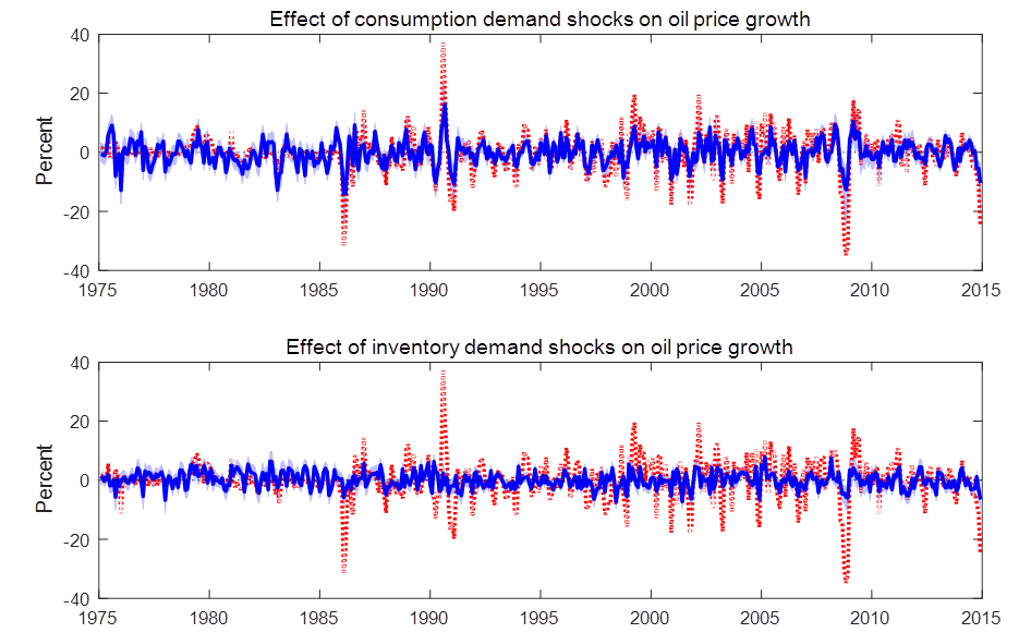
Red lines: actual monthly percent change in refiner acquisition cost for crude petroleum, 1975-2014. Blue lines and shaded regions: estimated contribution of indicated shock. Source: Baumeister and Hamilton (2015).
Again quoting from the paper:
Supply shocks were the biggest factor in the oil price spike in 1990, whereas demand was more important in the price run-up in the first half of 2008. All four structural shocks contributed to the oil price drop in 2008:H2 and rebound in 2009, but apart from this episode, economic activity shocks and speculative demand shocks were usually not a big factor in oil price movements. Interestingly, demand is judged to be a little more important than supply in the price collapse of 2014:H2.
We have drawn on a lot of prior information in producing the above graphs, though none of that information was used dogmatically as has been the case in previous studies. Another advantage of our approach is that we can examine what happens if we had considerably less confidence in any elements of the maintained prior beliefs. The last section of our paper explores the sensitivity of our main conclusions to such changes. We find that although our posterior credibility sets for most objects of interest would be wider when we have less faith in any specified components of the Bayesian prior, most of our broad conclusions would still emerge. For example, we did not find any specification for which there is more than a 2.5% posterior probability that supply shocks accounted for more than 2/3 of the cumulative oil price decline in the second half of 2014.
Prior information has played a key role in every structural analysis of vector autoregressions that has ever been done. Typically prior information has been treated as “all or nothing”, which from a Bayesian perspective would be described as either dogmatic priors (details that the analyst claims to know with certainty before seeing the data) or completely uninformative priors. In this paper we noted that there is vast middle ground between these two extremes. We advocate that analysts should both relax the dogmatic priors, acknowledging that we have some uncertainty about the identifying assumptions themselves, and strengthen the uninformative priors, drawing on whatever information may be known outside of the dataset being analyzed.
We illustrated these concepts by revisiting the role of supply and demand shocks in oil markets. We demonstrated how previous studies can be viewed as a special case of Bayesian inference and proposed a generalization that draws on a rich set of prior information beyond the data being analyzed while simultaneously relaxing some of the dogmatic priors implicit in traditional identification. Notwithstanding, we end up confirming many of the conclusions of earlier studies. We find that oil price increases that result from supply shocks lead to a reduction in economic activity after a significant lag, whereas price increases that result from increases in oil consumption demand do not have a significant effect on economic activity. We also examined the sensitivity of our results to the priors used, and found that many of the key conclusions change very little when substantially less weight is placed on various components of the prior.
https://research.stlouisfed.org/fred2/graph/fredgraph.png?g=295G
https://research.stlouisfed.org/fred2/graph/fredgraph.png?g=295B
https://research.stlouisfed.org/fred2/graph/fredgraph.png?g=295I
https://research.stlouisfed.org/fred2/graph/fredgraph.png?g=295L
https://research.stlouisfed.org/fred2/graph/fredgraph.png?g=295Q
https://research.stlouisfed.org/fred2/graph/fredgraph.png?g=295T
1. Think it is valuable to learn about elasticities and shapes of supply/demand curves (even the segments of them) and disentangle some of these variables.
2. Concerned if the sign concept is a recent aha from someone’s papers. Seems like micro econ 101 concept. Have stated it in comments for instance (‘if volume is up and price down, supply curve must have gotten cheaper. You could have some shifts of the demand curve also. But it’s impossible for demand alone to drop price, while volume is steady or increasing. (I.e. you can’t blame the failure of hundred here to stay on demand dropping…note volume is NOT even down, on any metric: refiner consumption or producer sales (i.e. storage at tank farms does not change the sign).
https://upload.wikimedia.org/wikipedia/commons/thumb/7/7a/Supply-and-demand.svg/1000px-Supply-and-demand.svg.png
3. Hard for me to say if Bayesian framework is really helpful/needed to do good analysis here. I sort of suspect that the (very useful) elucidations and examinations of elasticities can be done just as well without Bayesian considerations, but I am not an expert and these questions become philosophical/fashionable quickly.
4. Wonder how the forward looking nature of price is considered in these models. For a thought example consider a year ahead prediction of a project coming on line (or the converse). Right after the news is public, there will be a shift in price but nothing has changed in the producer costs of production and geologic constraints or in consumer demand for refined products. (it’s really speculator/tank farm/intermediary demand shifting).
A. If Q stays equal and P drops, than the supply curve must have gotten cheaper and the demand curve less needy, (the lines moved down together at same pace.
B. Still think a big lowering of the supply curve is notable, especially given the history of this blog and your writings which did not recognize the shale boom as it was ramping up and which have featured many references to prominent peak oilers like David Hughes, Art Berman, and Stuart Staniford (e.g., his 2007 Ghawar worries).
C. As a thought experiment, consider where P and Q would have ended up with whatever your model is of supply and demand, had demand curve remained same but supply curve made the shift you think it did (just interesting to see how different world would look.
D. Anecdotal evidence I hear is that the Chinese are still buying high volumes of oil. Any evidence that it has actually decreased?
E. If the demand curve dropped in concert with the supply curve (as in A), I wonder if that is all the countries dropping their curves at same pace or some more than others (the China concern). A first approximation way to look at this would be comparison amongst the countries for volume change. I.e. world volume is constant (by scenario), so if some countries are dropping volume and others increasing it, post price change (to net to zero), it implies demand curves dropping (more) in the countries with lower volume and less (or perhaps staying fixed) in the countries that had volume increases.
Almost forgot: time lag for production response is a nice idea to try to disentangle elasticities. Just a couple limitations:
a. OPEC, in particular, SA.
b. shutins (they actually happen for NG in the Marcellus, around 1.50 Transco hub price.)
Interesting exercise. As implied, a lot of expensive overhead for meagre results on the margin.
What happens when this model is run with quarterly data?
And within the world of academic economists, are quantities ‘demanded’ and ‘consumed’ really synonyms? Should they be? That is a nit-pick. Or is it? What exactly is ‘consumption demand’? For example. Is ‘demand’ now insufficient or somehow devoid of full meaning? Maybe the usage is evolving and I am not on top of it.
Monthly EIA US Crude + Condensate (C+C) data (the short term energy report) show a decline in US production from 9.6 million bpd in May to 9.0 million bpd in September. The annualized exponential rate of decline, based on May to September data, would be about 20%/year. If this (net) rate of decline were to continue for another year, US C+C production would be down to about 7.4 million bpd in September, 2016.
Louisiana is an interesting case history. As drilling activity declined in the Hayneville Shale Gas Play, gas production from the play production initially continued to increase (as operators worked through the backlog of drilling but uncompleted wells), but production from the play ultimately showed a sharp decline, with annual marketed natural gas production falling at a rate of 20%/year from 2012 to 2014. Measured from the monthly peak in December, 2011, it took about two and a half years for the exponential rate of decline in Louisiana’s monthly marketed gas production (from both shale gas + conventional production) to fall below 20%/year. The three year 12/11 to 12/14 rate of decline was 18.5%/year.
Regarding one of life’s little ironies, we keep hearing that oil exports from a net oil importer, the US (with recent four week running average net crude oil imports of 6.8 million bpd), will have a meaningful impact on global oil markets, just as the US is currently showing a 20%/year annualized rate of decline in C+C production, implying that US net oil imports will be increasing in the months ahead, if the production decline continues.
And the question that I have periodically posed, to-wit:
If it took trillions of dollars in global upstream capex to keep us on an “Undulating Plateau,” in actual global crude oil production (45 and lower API gravity crude, i.e., the quantity of the stuff corresponding to WTI & Brent oil prices), what happens to global crude oil production going forward given the ongoing cutbacks in global upstream capex?
Re: US Crude and/or Condensate Exports
As noted above, it’s more than a little ironic that there are so many claims that oil exports from a net oil importer, the US, will have a material impact on global oil markets, even as US Crude + Condensate (C+C) production is declining.
In any case, I just noticed something very interesting in the EIA Annual Energy Review data tables, which provide monthly and/or annual data back to 1950:
http://www.eia.gov/totalenergy/data/monthly/pdf/sec3_3.pdf
Note that US total liquids net imports were up year over year, from 4.9 million bpd in August, 2014 (2014 annual average of 5.1) to 5.6 million bpd in August, 2015, a 14% year over year increase in net total liquids imports.
Saw some analyst meeting (Genscape maybe) where the person projected rigs continuing to drop through 1Q16, ending up 200 more down (or about 400 remaining). This was based on prices staying in this ~$47-50 band, with commensurate strip. [A drop down to ~$40, with commensurate strip would lead to an additional 200 rigs going away.]
I think the Haynesville is a nice example to show the “lag” effect when rigs drop. And really, we can already use the US oil production as an example of this already. Another easy example is 2009 in the Bakken.
I would be leery of thinking too much that the Haynesville is some sort of example of Hubbert peak because a lot of the drop is price caused, not exhaustion. [In a classic Hubbert peak case for global oil or national gas, you would have the normal curve AND would have Hotelling price increase. In this case, it’s not even constant price…it’s reaction to a price crash.] Haynesville didn’t drop because “they ran out of sweet spot” but because the price dropped. There is actually more resource available, now, if we go back to previous prices…because of improvements in drilling and completion efficacy. [This is Adelman’s point of how you don’t just eat away at lower cost oil and move to higher…yes, you may be doing that. But in addition, knowledge can grow the pool of available low cost oil or reduce the price of getting out what you already know about. Both effects can occur and they fight each other and you have to get into the specifics to see which is winning.]
In addition, concentrating on the Haynesville, when the Marcellus and Utica have occurred is missing the main story from an economic impact perspective. After all, volume is up and price is down for natural gas. So for all the H or the B dropped, the M and U more than made up for it. “The App” is the key place to look at in US natural gas.
In addition, FWIW, H did drop very beautifully in a Hubbert-like manner from the peak of 7, BUT for the last 18 months has been near flat at 4 BCF/day. Download the excel data (last figure at bottom of page) and graph it and you will see that. Peak oilers discussing the Haynesville as some sort of organic product life cycle analogy (born, grow, mature, die), never mention this key insight (how it has flattened out dramatically now). But it’s in the data. Just graph to see it.
http://www.eia.gov/naturalgas/weekly/ (note this shows the shale only, not the conventional production. EIA DPR as a data source makes the fat tail look even more prominent, but includes conventional in the region.)
So, given the right price incentives, the sum of the output of discrete sources of oil & gas–that individually peak and decline–will never peak and decline?
In any case, in regard to price versus production, we have an interesting case history when it comes to actual crude oil production (generally defined as 45 API and lower crude oil). Following is an essay, which I sent to some industry acquaintances a few weeks ago:
Regarding oil prices, I may be one of the worst prognosticators around, especially when it comes to demand side analysis. My primary contribution has been as an amateur supply side analyst, especially in regard to net exports.
In any case, earlier this year I thought that we had hit the monthly low in Brent prices for the current oil price decline ($48 monthly average in January, 2015), and I thought we were more or less following an upward price trajectory, from the 1/15 low, similar to the price recovery following the 12/08 monthly oil price low ($40 for Brent).
However, a key difference between the 2008/2009 price decline and subsequent recovery and the 2014/2015 decline is that Saudi Arabia cut production from 2008 to 2009 while they increased production from 2014 to 2015.
But for what it’s worth (perhaps not much), I think that this is a tremendous buying opportunity, in regard to oil and gas investments. I don’t have any idea what Warren Buffet is doing right now, but I would not be surprised to learn that he is aggressively investing in oil and gas.
The bottom line for me is that depletion marches on.
A few years ago, ExxonMobil put the decline from existing oil wells at about 4% to 6% per year. A recent WSJ article noted that analysts are currently putting the decline from existing oil wells at 5% to 8% per year (in my opinion, the 8% number is more realistic). At 8%/year, globally we need about 6.5 MMBPD of new Crude + Condensate (C+C) production every single year, just to offset declines from existing wells, or we need about 65 MMBPD of new C+C production over the next 10 years, just to offset declines from existing wells. This is equivalent to putting on line the productive equivalent of the peak production rate of about thirty-three (33) North Slopes of Alaska over the next 10 years.
It appears quite likely that global crude oil production (45 and lower API gravity crude oil) has been more or less flat to down since 2005, as annual Brent crude oil prices doubled from $55 in 2005 to $110 for 2011 to 2013 inclusive (remaining at $99 in 2014)–while global natural gas production and associated liquids, condensate and NGL, have (so far) continued to increase.
Following are links to charts showing normalized production values for OPEC 12 countries and global data. The gas, natural gas liquids (NGL) and crude + condensate (C+C) values are for 2002 to 2014 (except for gas, which is through 2013, EIA data in all cases). Both data charts show similar increases for gas, NGL and C+C from 2002 to 2005, with inflection points in both cases for C+C in 2005. My premise is that condensate production, in both cases, accounts for virtually all of the post-2005 increase in C+C production.
Global Gas, NGL and C+C:
http://i1095.photobucket.com/albums/i475/westexas/Global%20Gas%20NGL%20C%20amp%20C_zpskb5bxu6d.jpg
OPEC 12 Gas, NGL and C+C:
http://i1095.photobucket.com/albums/i475/westexas/OPEC%20Gas%20NGL%20C%20amp%20C_zpsox3lqdkj.jpg
Currently, we only have crude oil only data for the OPEC 12 countries and for Texas (note that what the EIA calls “Crude oil” is actually C+C).
Also following is a link to OPEC 12 implied condensate (EIA C+C less OPEC crude) and OPEC crude only from 2005 to 2014 (OPEC data prior to 2005 was for a different set of exporters than post-2005). Obviously, data quality is an issue, and the boundary between actual crude and condensate is sometimes fuzzy. In any case, we have to deal with the data that we have.
OPEC 12 Crude and Implied Condensate:
http://i1095.photobucket.com/albums/i475/westexas/OPEC%20Crude%20and%20Condensate_zps12rfrqos.jpg
As of 2014, OPEC and the US accounted for 53% of global C+C production (41 MMBPD out of 78 MMBPD). Implied OPEC condensate production increased by 1.2 MMBPD from 2005 to 2014 (1.2 to 2.4). The EIA estimates that US condensate production increased by about 1.0 MMBPD from 2011 to 2014. I’m estimating that US condensate production may have increased by around 1.2 MMBPD or so from 2005 to 2014. Based on the foregoing, increased condensate production by OPEC and the US may have accounted for about 60% (about 2.4 MMBPD) of the 4 MMBPD increase in global C+C production from 2005 to 2014.
Combining the US and OPEC estimates, the US + OPEC ratio of condensate to C+C production may have increased from about 4.6% in 2005 to about 10% in 2014. If this rate of increase in the global condensate to C+C ratio is indicative of total global data, it implies that actual global crude oil production (45 and lower API gravity) was approximately flat from 2005 to 2014, at about 70 MMBPD.
In other words, the available data seem quite supportive of my premise that actual global crude oil production (45 API and lower gravity crude oil) effectively peaked in 2005, while global natural gas production and associated liquids, condensate and NGL, have (so far) continued to increase.
If it took trillions of dollars of upstream capex to keep us on an “Undulating Plateau” in actual global crude oil production, what happens to crude production given the large and ongoing cutbacks in global upstream capex?
And given the huge rate of decline in existing US gas production (probably on the order of about 24%/year from existing wells), it’s possible that we might see substantially higher North American gas prices this winter, given the decline in US drilling.
Furthermore, through 2013 we have seen a post-2005 decline in what I define as Global Net Exports of oil (GNE, the combined net exports from the Top 33 net exporters in 2005), which is a pattern that appears to have continued in 2014. GNE fell from 46 MMBPD in 2005 to 43 MMBPD in 2013 (total petroleum liquids + other liquids). The volume of GNE available to importers other than China & India fell from 41 MMBPD in 2005 to 34 MMBPD in 2013.
Here are the mathematical facts of life regarding net exports:
Given an ongoing, and inevitable, decline in production in the net oil exporting countries, unless the exporting countries cut their liquids consumption at the same rate as, or at a faster rate than, the rate of decline in production, the resulting rate of decline in net exports will exceed the rate of decline in production and the net export decline rate will accelerate with time.
In addition, while we are currently seeing signs of weak demand in China, given an ongoing, and inevitable, decline in GNE, unless China & India cut their net oil imports at the same rate as, or at a rate faster than, the rate of decline in GNE, the rate of decline in the volume of GNE available to importers other than China & India will exceed the rate of decline in GNE, and the rate of decline in the volume of GNE available to importers other than China & India will accelerate with time.
For example, from 2005 to 2013 the rate of decline in the volume of GNE available to importers other than China & India (2.3%/year) was almost three times the observed rate of decline in GNE from 2005 to 2013 (0.8%/year).
And a massively under-appreciated aspect of what I call “Net Export Math” is that the rate of depletion in the remaining cumulative volume of net oil exports, after a net export peak, tends to be enormous. Saudi Arabia is showing a year over year increase in production and net exports, but based on available annual data through 2014, Saudi Arabia’s net exports fell from 9.5 MMBPD in 2005 to 8.4 MMBPD in 2014 (total petroleum liquids + other liquids), and I estimate that Saudi Arabia may have already shipped close to half of their total post-2005 supply of cumulative net exports of oil.
“So, given the right price incentives, the sum of the output of discrete sources of oil & gas–that individually peak and decline–will never peak and decline? ”
So again, the argument for imminent decline is some eventual limit to the amount of hydrocarbons on the entire planet? it is not cherrypicking to emphasize the Haynesville and Barnett as gas plays “peaking” when overall gas production in the US has grown 40%, even in the face of a huge price drop????
“In any case, in regard to price versus production, we have an interesting case history when it comes to actual crude oil production (generally defined as 45 API and lower crude oil).”
Nope. Lease condensate (~55) is legally considered crude oil. EF 47 is a normal listed form of oil in Platts price lists. Light oil and condensate is used to make gasoline and other products and runs through a refinery. It is easily and routinely blended with heavy oil and is actually needed for that (not just as a diluent for transport but for optimizing the subunits of complex refinery (non complex refineres, e.g. those without cokers or visbreakers or with less cracking actually function better on just light blends to start…the extreme are teakettle refineries).
Condensate and EF crude is withing a few dollars of WTI and correlates with price moves very closely. EF 47 is actually pricier than heavy sour crudes. Talk to any trader, refinery buyer, or even just a microeconomist familiar with looking at substitutes. It is crazy to say that growth of 45+ oil has not affected overall oil prices. Perhaps some small shrinking of spreads between qualities, but often not even a directionality change. The much larger impact though is on the overall supply demand balance for C&C. Does any economist think the goods are sufficiently different to justify a separate P-Q curve for 45- and 45+ oil? [Oh…and the extra funny thing is the peak oil meme of mid 2000s was that we wouldn’t find more light sweet!]
P.s. If you really think 45+ isn’t oil, then why not agree to remove the export restriction on at least them?
“Following is an essay, which I sent to some industry acquaintances a few weeks ago:”
Your cut and pasting the things on the net (ELM stuff, net export arguments) is almost spammy. Total conversation killer and often ignored by even your compatriots.
Nony: You make good arguments for lumping crude oil and condensates.
The problem with a net export perspective is that it ignores the global nature of the market place and at some point, an indifference to whether heavy oil imported into the US refinery complex hails from western Canada, Venezuela, Mexico or Colombia. Or even Iran some day.
If we could draw and compare distribution curves of oil grades over the last , I suspect we would see the distributions flattening out over time as extreme grades become more prominent. It may even be bi-modal at this point.
Given the expense of retooling refineries and the robust growth in US condensate production, one can see the interest in securing more pipeline access to Canadian bitumen. And perhaps the interest in hoping/praying for growth in Colombian heavy oil production as Mexican production declines and the populist Neo-Marxist experiment in Venezuela violently implodes stagnating heavy oil production in that country.
Jeffrey Brown: I don’t want to suggest that the net export perspective is not useful. It clearly illustrates symptoms of the Resource Curse and the general difficulty experienced by citizens in weak societies to play and cooperate well together. It does not however say much about the US cheap energy entitlement and how that attitude has hurt US national security and economic performance over time. America’s well earned reputation for killing grandchildren and grandparents in part stems from this ill-advized quest for cheap energy security (sic).
Erik,
I’m not arguing the relative merits of crude oil versus condensate, although distillate yield begins to drop off precipitously over an API gravity of about 40 or so.
I am arguing that the available data strongly suggest that global crude oil production probably peaked in 2005, while global natural gas production and associated liquids, condensate and natural gas liquids, have (so far) continued to increase.
In regard to net oil exports, here’s the problem: Given an ongoing, and inevitable, decline in production in a net oil exporting country, unless they cut their liquids consumption at the same rate as, or at a faster rate than, the rate of decline in production, it’s a mathematical certainty that the resulting rate of decline in net exports will exceed the rate of decline in production and that the net export decline rate will accelerate with time.
I don’t think it makes economic sense to put lease condensate with NGLs and away from crude. NGLs are more gas like, so you can put them with gas if you want instead of oil or just make a third grouping. [But don’t forget them! If you cut the total liquid products to being C&C, they still belong somewhere…have use!]
NGLS are mostly (c2-c4) molecularly pure, separated, gaseous products. [minor amount of C5+ liquid (“plant condensate” obtained at the gas refrigeration separation plant].
Lease condensate is just the associated entrained liquid oil from a primarily gas well. It is obtained at the atmospheric, three phase separator at the wellhead. Similarly, wet gas is separated from predominantly oil streams. Eagle Ford 47 isn’t even coming out of “gas wells” (in terms of phase) but single phase liquid oil wells that are very light. Lease condensate and Eagle Ford 47 look like oil, smell like oil, mess up your Nomex coveralls in a similar manner to 30 API oil. They are each that glorious natural product that contains a soup of hundreds of different molecules, of different lengths, aromaticities, branching. Oh and less sulfur (which makes them BETTER oil) but still with some. Lease condensate also tends to be a bit lower API and more variable in composition versus plant condensate (although higher than oil), but still pretty similar.
There is a reasonable argument to exclude NGLs entirely from crude time series or at least C3 and C2 from being lumped in with crude. Ethane in theory competes with naphtha and is an occasional substitute (and some crackers are convertible), but given the glut, prices have diverged and started to follow C1 a couple years ago. And like C1, it is quite difficult to transport across oceans. C3 is more exportable, but still has a pretty different market (mostly heating) than premium liquid petroleum products (mostly transport fuels: gasoline, diesel, jet). [In a sense, C1 is a substitute for oil, but it’s a pretty weak substitute!]
So yeah, sure, strip out the NGLs. And throw in the C4 and C5+ with being stripped out, since they are minor…even though ARE mostly used for transport. Either direct gasoline mixing for butane or for C5+ mixed into crude (at refineries or upstream at heavy oil sites) or used as naphtha in crackers (thus competing with a refined liquid stream. But fine keep them all apart.
But keeping condensate (or Eagle Ford 47 oil) apart from other grades of crude makes no sense. That stuff goes through refineries and makes gasoline…a lot of gasoline, which is generally what the refinery is optimized for. (Other products have value and you go for a global optimum, not a local. Like you don’t optimize production of RFO and make little gasoline! Diesel and jet have value of course and at times, pricing of diesel can beat out gasoline, but generally gasoline is top in both value. And certainly in volume (typical refinery cracks some product that could have been diesel to make more gasoline). Just look at Platts prices and the correlation of EF47 and DJ condensate versus WTI. It’s the same stuff, but slightly different flavors, man. If you look at it on a world basis (where the explosion of light and super light is export-ban trapped on a continent that wants to refine 28 API), the correlations will be even stronger. But I bet even in the US, you find a very consistent correlation: maybe just look at annual average prices for 2008, 2009, 2014 and 2015 YTD. Condensate belongs with crude, from a supply-demand standpoint. Not with NGLs or with NG.
Here’s a link showing Saudi 50 API crude selling in the same setting as other grades of crude (i.e. considered a similar good, not considered an NGL). AND at a premium to medium grade Gulf oil. AND even at a greater premium than other light, but less light oils.
http://www.bloomberg.com/news/articles/2014-05-04/saudi-aramco-raises-all-june-crude-price-differentials-to-u-s- [scroll down to the header “Asia”]