Today, we are pleased to present a guest contribution written by Fabrizio Venditti (European Central Bank) and Giovanni Veronese (Banca d’Italia). The views expressed in this paper belong to the authors and are not necessarily shared by the Banca d’Italia and the European Central Bank.

---

The oil market was one of the timeliest gauges of the effect of the Covid-19 shock on global activity. Between February and April 2020 the price of crude plummeted. Containment measures and travel bans resulted in an unprecedented collapse of the demand for oil. On the supply side the market was also shaken by faulty strategic interactions among the main producers. OPEC+, the coalition of major non-US producers led by Saudi Arabia and Russia that had successfully curtailed supply since 2016, unravelled over a fundamental disagreement on how to respond to collapsing demand and initiated a price war. Excess production flowed into inventories, which quickly filled up global storage capacity. In April, storage demand at Cushing Oklahoma became so extreme that futures WTI prices settled at negative prices for the first time in history. Eventually OPEC and Russia in April agreed to initiate production cuts as of the 1^st of May, although the International Energy Agency (IEA) does not expect these cuts to be sufficient to rebalance the market any time soon (Figure 1).

Figure 1: Oil production and consumption
(year-on-year percentage changes)

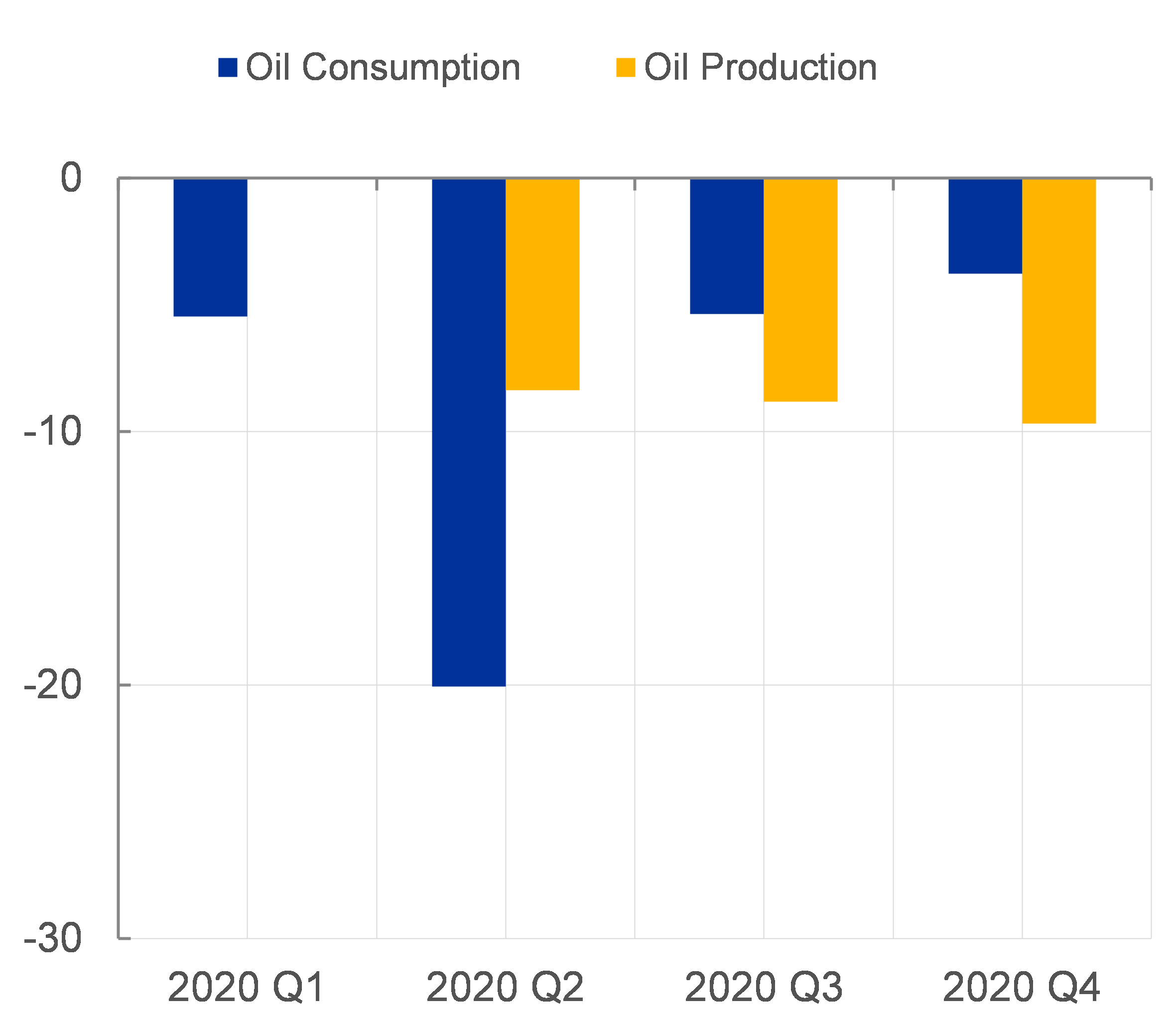
Sources: International Energy Agency (IEA). Notes: estimates from the May Oil Market Report.

 Disentangling the structural drivers of the price of oil is crucial both for policy makers as well as for market participants. First, oil is an important input into economic production and sustained (supply driven) price increases can throw the global economy into recession (Kanzig, 2020). Second, oil prices impact directly inflation and consumer spending through energy prices, as oil prices are passed on (one to one) to gasoline prices within a week (Venditti, 2013). Third, commodity prices, move strongly in sync with the global business cycle (Delle Chiaie, Ferrara and Giannone, 2017). Finally, in recent years, oil has become an important financial asset. However, the models that are most frequently used for assessing the structural drivers of oil prices typically rely on low-frequency variables that are only available with a substantial delay. As a result, these models typically paint an outdated picture of the state of the economy, and are not particularly useful when more timely information is needed. In a recent paper (Venditti and Veronese, 2020) we develop a new method for decomposing the price of oil into its structural drivers in real time at the daily frequency, exploiting the relationship between oil prices and global financial markets. Using a daily structural Vector Autoregression (VAR), in which we jointly model spot and futures oil prices as well as stock prices, we decompose the price of oil in three structural shocks. The first shock is a forward looking demand shock, which captures the impact on the oil price of changes in expectations about future economic activity. We label this shock, risk sentiment shock, as it embodies unexpected changes in the risk sentiment of market participants on the outlook of global activity. The second shock is an unexpected change in the current state of the business cycle and, as a consequence, in commodities demand more broadly. The third shock is a supply shock, which captures but current and expected changes in oil supply.

The model offers insights on the behaviour of the price of oil during the Covid-19 crisis and on the interaction between oil prices and financial markets. Figure 2 shows how the model decomposition of oil price into its structural drivers between mid-February and the 25^th of May 2020. According to the model, the collapse of the price of oil between February and April is entirely due to the concurrent fall in demand for oil, as well as to tumbling risk sentiment (respectively, yellow and blue bars). The contribution of supply is rather erratic until the end of April, amid uncertainties on the negotiations between Russia and Saudi Arabia. Since the end of April, as lockdown measures start being relaxed, demand shocks lead a recovery of the price of crude. Supply contributes to this trend, as production cuts implemented by the OPEC+ coalition, as well as shut-ins of oil wells in the US as well as in Canada, begin having an effect on prices. Interestingly risk shocks, which we interpret as longer term growth expectations, keep exerting downward pressure on crude prices, indicating that the market does not expect a swift economic recovery out of the Covid recession.

Figure 2: Oil price decomposition
(daily cumulated percentage change since 21/2/2020)

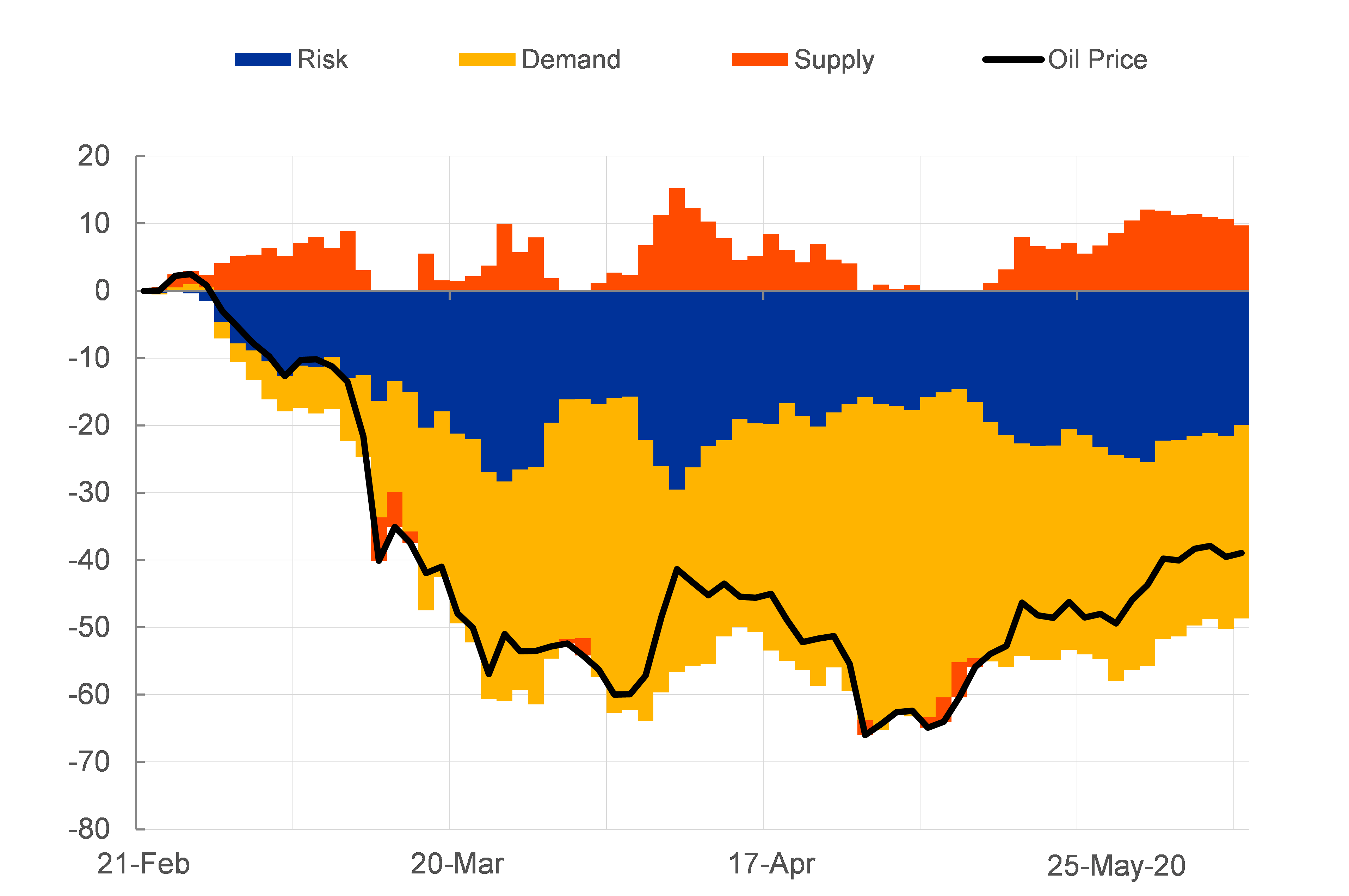
Sources: Datastream and authors calculations. Notes: structural shocks are estimated using the spot and futures oil prices and the global stock index of airlines. For details see Venditti and Veronese (2020). Percentage changes as approximated by log changes are adjusted in order to address the large scale of the oil price movements.

According to our oil market model, the Covid-19 shock will persistently depress global activity. This will have deflationary implications, not likely to dissipate any time soon, something flagged also by the developments in the inflation swap markets. Both in the euro area as well as in the US, 5-year/5-year forward inflation-linked swap rates, a popular measure of market based inflation expectations, have fallen markedly since the beginning 2020. In Figure 3 we plot them together with the contribution of the risk shock to the price of oil as estimated in our model. The correlation since 2019 is remarkably tight, especially for the euro area.

Figure 3: Inflation expectations and oil price risk shocks
(lhs: inflation expectation; rhs: risk shock; percentage points and contribution to cumulated log changes)

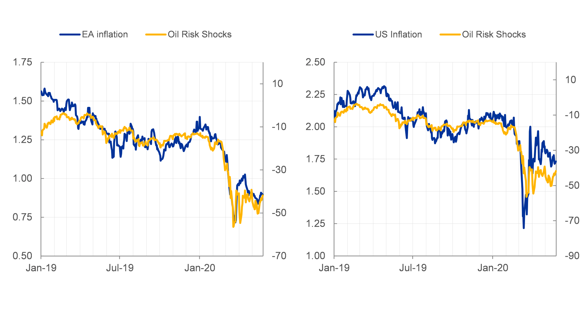
 Sources: Bloomberg and authors calculations. Note: Oil risk shock series is the contribution of risk shocks in the historical decomposition of the price of oil, coming from our daily model. In the model the price of oil is transformed in logs and multiplied by 100.

Conclusions

The Covid-19 shock has shaken the global oil markets, leading to an unprecedented supply glut, amid a temporary price war between oil producers. Understanding in real time the relative role of demand and supply in shaping oil prices is challenging, as hard data on oil production and on global economic activity are released only with a delay. We use a model based on financial asset prices to bridge this information gap and shed some light on the structural drivers of oil prices in times of Covid-19. Our results suggest that supply played overall a limited role in the oil price slump. Most of the oil drop was due to the effect of containment policies on energy demand and to investors’ pessimism about longer term global economic prospects.

 

Kanzig, D. (2018), “The Macroeconomic effects of oil supply news: evidence from OPEC announcements” available at https://ssrn.com/abstract=3185839.

Venditti, F. (2013) “From oil to consumer energy prices: How much asymmetry along the way?“, Energy Economics, Elsevier, vol. 40(C), 468- 473.

Delle Chiaie, S., Ferrara, L. and Giannone D. (2017), “Common factors of commodity prices”, Banque de France Working Paper No. 645.

Venditti, F. and Veronese, G.(2020), “Global Financial Markets and Oil Price Shocks in Real Time”. ECB Working Papers, forthcoming. Available at SSRN: https://ssrn.com/abstract=3577551.

---

This post written by Fabrizio Venditti and Giovanni Veronese.