Today’s two sessions — one in the NBER’s International Finance and Macro group and one in Monetary Economics — included papers that tackled multipliers from a variety of directions. The general results indicated to me that, while multipliers are sometimes below unity, for conditions prevailing in the United States in 2011, they are typically above.
The first paper, by Ethan Ilzetzki, Enrique Mendoza, and Carlos Vegh, entitled “How Big (Small?) are Fiscal Mutlipliers?”, too a cross country view, applying panel regressions and panel VARs to the question. From the abstract:
We contribute to the intense debate on the real effects of fiscal stimuli by showing
that the impact of government expenditure shocks depends crucially on key country
characteristics, such as the level of development, exchange rate regime, openness to
trade, and public indebtedness. Based on a novel quarterly dataset of government
expenditure in 44 countries, we find that (i) the output effect of an increase in gov
ernment consumption is larger in industrial than in developing countries, (ii) the fiscal
multiplier is relatively large in economies operating under predetermined exchange rate
but zero in economies operating under flexible exchange rates; (iii) fiscal multipliers
in open economies are lower than in closed economies and (iv) fiscal multipliers in
high-debt countries are also zero.
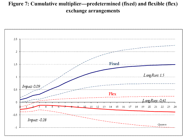
The authors obtain their findings in part using stratified samples. One key result — that the multiplier is larger in cases where the exchange rate is fixed — is illustrated in Figure 7.

Figure 7 from Ilzetzki et al (2011).
Why is the multiplier larger for countries fixed exchange rates? One interpretation, consistent with the Mundell-Fleming model (under high capital mobility) is that expansionary fiscal policy is more accommodated under pegged rates; the authors find that monetary policy is indeed more accommodative under fixed rates.
Paul Krugman has interpreted this finding as applying to the United States, to the extent that the Fed is pursuing an accommodative policy; and to the extent that we are at the zero interest rate bound for what appears to be indefinitely, given recent reports of economic weakness, that conjecture seems right to me.
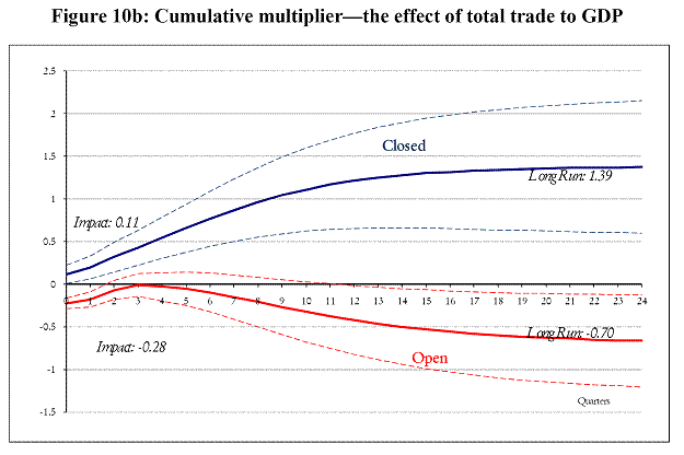
Another finding is that closed economies have larger multipliers, a result once again consistent with a Keynesian model. Figure 10b shows the IRF for the case when openness is measured by trade shares; in this case, as indicated in Table A5, the US is a closed economy, far below the threshold for the definition of openness. [add’l text added, graph changed from 10a to 10b 7;20 pm]

Figure 10b from Ilzetzki et al (2011).
In addition, if the countries are stratified by size (and the US is definitely large in this context), then once again the multipliers are larger in the large economies, in a manner consistent with Figure 10b. [add’l text added 7:20pm]
So, ask yourself — is the US a small country with the monetary authorities actively moving the interest rate around in order to respond to fiscal impulses; or is it better characterized as a large, relatively closed, economy with short interest rates at near zero. Then consider which results apply.
The next paper, by Emi Nakamura, and Jon Steinsson, entitled “Fiscal Stimulus in a Monetary Union: Evidence from U.S. Regions”, looked to intra-country data. From the abstract:
We use rich historical data on military procurement spending across U.S. regions to estimate
the effects of government spending in a monetary union. Aggregate military build-ups and
draw-downs have differential effects across regions. We use this variation to estimate an open
economy relative government spending multiplier of approximately 1.5. We develop a framework
for interpreting this estimate and relating it to estimates of closed economy aggregate multipliers.
The closed economy aggregate multiplier is highly sensitive to how strongly aggregate monetary
and tax policy “leans against the wind.” In contrast, our estimate “differences out” these effects
because different regions in the union share a common monetary and tax policy. Our estimate
provides evidence in favor of models in which demand shocks can have large effects on output.
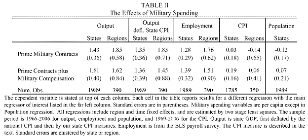
The basic empirical results are summarized in Table II of the paper:

Table II from Nakamura and Steinsson (2011).
Finally, in the last paper, Price Fishback, and Valentina Kachanovskaya go back in time, in “In Search of the Multiplier for Federal Spending in the States during the New Deal”. From the abstract:
If there was any time to expect a large peace-time multiplier effect from federal
spending in the states, it would have been during the period from 1930 through 1940.
Interest rates were near the zero bound, and unemployment rates never fell below 10
percent and there was ample idle capacity. We develop an annual panel data set for the
48 states from 1930 through 1940 with evidence on federal government grants, loans, and
tax collections and a variety of measures of economic activity. Using panel data methods
we estimate a multiplier, defined as the change in per capita economic activity in
response to an additional dollar per capita of federal funds. The state per capita personal
income multiplier with respect to per capita federal grants was around 1.1. Some point
estimates for multipliers for nontransfer grants and nonfarm grants were higher but not
statistically significantly different from one. There is some evidence that AAA farm
grants had negative or no effect on personal income. Federal grants had stronger effects
on consumption than on personal income, but they had no positive effect on various
measures of private employment.
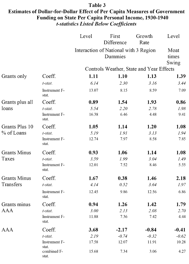
Key results are presented in Table 3.

Table 3 from Fishback and Kachanovskaya.
The empirical results were dispersed, and in my opinion one particularly important drawback of the analysis is the use of state income as the dependent variable. Ideally, one would want gross state product, analogous to the national-level gross domestic product, but the data are the data, and one has to work with what one has.
I would tend to focus on the results under the column labeled “growth rates”, as first log differencing should eliminate trend effects. What we see there is that the point estimates are above unity (except for AAA payments which are aimed at reducing crop production).
What I take from these papers’ empirical results is that the proposition that multipliers are positive and (for government consumption and/or investments) in excess of unity, for conditions most applicable to the United States. This charactization is in line with the my (many) earlier posts on the subject of multiplier, which are collected here.
I’m sorry if you’ve addressed this already, but we seem to get hung up on how much more than 1 the multiplier may be when the real issue, it seems, is whether it is 1 or below. The government is, in a tough time, taking on debt to prop up consumption, services, production so, to me, while it’s nice that the multiplier be over 1, all that really matters – again, to me – is that the multiplier not be below 1. If the money is just money with no additional effect then it still does the job.
So, ask yourself — is the US a small country with the monetary authorities actively moving the interest rate around in order to respond to fiscal impulses; or is it better characterized as a large, relatively closed, economy with short interest rates at near zero. Then consider which results apply.
Unfortunately, that is not how it works. If you are going to interpret Ilzetzki’s results you must use their definition of open and closed. And according to the table you have presented, the U.S. is an open economy.
By the way, was there any reason why you neglected to mention their other finding that fiscal stimulus may be counter productive during periods of high debt-to-GDP ratios (>60%)?
Paul Krugman has interpreted this finding as applying to the United States, to the extent that the Fed is pursuing an accommodative policy; and to the extent that we are at the zero interest rate bound for what appears to be indefinitely, given recent reports of economic weakness, that conjecture seems right to me.
Another finding is that closed economies have larger multipliers, a result once again consistent with a Keynesian model.
And not such good news if you’re a small country on Europe’s periphery.
Jeff: You are right that Figure 10a pertains to the de jure measure. However, Figure 10b (which is what I should have used, and will replace 10a with) indicates a situation in which the US has a higher multiplier. From page 18 of the paper:
If you then consult Table A5 on page, you will see the United States at 18.2%. The IRFs are based upon this definition.
To resolve this inconsistency, the authors re-estimate stratifiying by size (in which case obviously the US is large). In that case, the multiplier is larger for large countries (including the US). So I count two out of three for the US having larger multipliers.
I quoted the entire abstract. Even if the multiplier is smaller for high debt countries, the other attributes of the US push the multiplier larger (as I have described). I will also note that when the ARRA was passed, public debt to GDP was 0.486.
Evidence that the government spending multiplier is NEGATIVE …… from a group smarter than your typical Keynesian economist:
“A new Rasmussen Reports finds that 55% of likely U.S. voters believe that a decrease in government spending would help the economy.”
Short term vs. Long term. That is a key issue.
The current non-responsiveness of this economy to all variety of stimulative measures, unprecedented in scope, is a result of long term structural issues that were built up over approximately 25 years.
I am talking about total credit market debt. It seems that whenever debt comes up in discussion, people start freaking out.
One side says the US is not in that bad of shape, and there clearly is room to add more, and we clearly should do so to improve the immediate situation. This is because they look only at Federal Gov debt, as some % of GDP, and compare it to other data points throughout the ‘modern’ economic world.
The other side screams that the world is coming to an end, and we have to fix the problem now, which would of course plunge us into an immediate economic contraction.
But both sides fail to look at the big picture…and most economist types seem to as well. Is it not TOTAL ACCUMULATED DEBT (Federal + State/Muni + Corporate + Consumer + Mortgage) that matters?
If debt service is paid out of government tax revenues, and the country has just spent 20 years borrowing and spending the proceeds to fund their lifestyle, and pump up asset prices, instead of investing in value adding capital goods, etc, will not the ability of the country to earn economic profits to fund Federal level deficits be impacted? Of course they will.
The previous peak of total credit market debt to GDP was 270% in the Great Depression…and this only occurred because the economy collapsed so much faster than debts were being written off during that hard period. For most of the ‘normal’ phases of the 20th century, total credit market debt to GDP was between 120-160%. Today we are at 370%.
How can this not be acknowledged by anyone when issues of debt, monetary, and fiscal policy are discussed. It is of paramount importance.
The failure of economists, academics, and the Federal Reserve to view the accumulation of debt as a danger is a blunder of historic proportions.
The ‘bailouts’ of 2008 were based on this fantasy that we could somehow trick the economy into growing again by transferring all these private sector bad debts to the public. Well guess what…it is not working.
The current economic situation is a result of the failure of the American perspective. Our inability to think long term has put us here. For 25 years we have focused on the short term. Every time the economy had a recession, we turned the central bank loose to “fix” things in a monetarist frenzy.
There is a fundamental issue with this. What if nothing needed fixing!? Recessions are normal. They are part of a capitalistic system. Our belief that we must to everything to end every little patch of economic difficulty as soon as possible, without regards to the accumulation of debt is insane.
When you try to create an economy where everyone wins…we all eventually lose.
There are all sorts of measures that have been warning us for 15 years that this day was coming. Most important are the figures showing marginal increases in GDP relative to additions of debt (regardless of sector). This marginal productivity or debt has been on a straight path towards zero for a long long time…and yet no one noticed.
So now we are at this point where the accumulated total credit market debt is so high, that it does not matter any more how much we pump in. Massive amounts of credit infusion result in….. no growth.
We have spent the last 20+ years on an orgy of credit growth. It has enabled a financial sector to create this fantasy they finance and ‘brokering’ in general created economic growth, when in reality all the financial sector does is steal a portion of the stock of wealth of the nation because they are positioned to siphon gains from the massive credit infusions.
So many flawed ideas from academia have lead to this mess…and most can be traced back to the propensity of the economic establishment to pay no attention at all to the accumulation of total debt loads, and where we are in the inter-generations credit cycle that seems to peak and collapse every 70-80 years.
Every economics ‘sect’ has their strong and weak points, but the classical and Austrian schools certainly seem to be best suited to explain the trap we are in.
Unfortunately, when you ask them for a solution, they will tell you there is none. And I think they are right. The only question is how much worse will the politicians (and the economic advisers with their bogus econometric models based on flawed and inadequate sample sizes) make things.
Menzie: I will also note that when the ARRA was passed, public debt to GDP was 0.486.
So social security debt doesn’t matter eh? Gonna pay them SS recipients with government bonds from the lock box.
When the Spender in Chief passed ARRA, the ratio of total debt to GDP was well north of 70%.
It is not obvious that the fiscal multiplier is always providing for a continuous increased source of public revenues as evidenced by the graphs (Econbrowser,Detachment from Reality and Innumeracy as Impediments to Rational Discourse).It is obvious that the tax benefits through their mode of distribution may drive to a saturation effect.
(The Bush tax and the economy Congressional service Thomas L Hungerford)
Don’t forget private debt.
Paul Krugman has interpreted this finding as applying to the United States, to the extent that the Fed is pursuing an accommodative policy; and to the extent that we are at the zero interest rate bound for what appears to be indefinitely, given recent reports of economic weakness, that conjecture seems right to me.
Considering that the actual effect of QE2 on treasury yields was likely modest and easily overwhelmed by many other factors, this explanation seems a bit like an ex-post rationalization to fit ones world-view onto the data rather than an honest attempt to understand what’s going on.
Dave,
Total FEDERAL Gov debt was 70%. At that time…Total Credit Market Debt was in the range of 350%! You make the same mistake that I pointed out…everyone forgets about private sector debt, and state/muni debt. It all matters. If TOTAL debt to GDP in the US were only 70%, we would not be in this mess!
ppcm,
Thanks for chiming in on private debt….
No econometric model on earth has ANY validity right now, because we have never had this amount of total debt. This is why economists keeps getting it wrong. They think that they have valid data from which to curve fit…but they do not. They have nothing, because from about 1992 onward…we have been in uncharted territory as to debt to GDP….and from 2007 on..we have been at debt saturation…something the Austrians seems only to see…
I’m sure that, even as I type this, Robert Barro is burning the midnight oil trying to prove that the world is, in fact, flat…..
The rate could be fixed to disguise the decline in real purchasing power. After all, if the floating rate indicates stability or increasing value, why fix it at all?