The 30th Annual International Symposium on Forecasting was held in San Diego last week. Among the many interesting presentations was Princeton Professor Mark Watson’s discussion of estimating business cycle turning points using a large number of indicators.
Watson began his talk by reviewing some of the history of how the approach to assigning business cycle dates has evolved over time. The designations of U.S. recessions prior to World War II are based on the work by Arthur Burns and Wesley Mitchell, who looked at close to a thousand separate indicators and identified by eye what appeared to be “peaks” and “troughs” in each series, one by one. Burns and Mitchell then tried to summarize this set of sector-specific dates in terms of episodes during which a large number of indicators moved down together, categorizing series further in terms of whether they were leading and lagging indicators relative to those aggregate tendencies and the degree of procyclicality or countercyclicality of each individual series.
After World War II, business cycle dating was carried on by Geoffrey Moore and Victor Zarnowitz. They identified separate turning points for each of a few dozen indicators, and again sought to harmonize these to obtain reference cycle dates. Dating by the NBER Business Cycle Dating Committee gradually evolved into the present focus, in which it is the behavior of aggregate economic indicators that is taken to be the focus of the inquiry. For example, Watson quoted from the December 2008 press release of the NBER’s Business Cycle Dating Committee:
Because a recession is a broad contraction of the economy, not confined to one sector, the committee emphasizes economy-wide measures of economic activity. The committee believes that domestic production and employment are the primary conceptual measures of economic activity.
Watson and coauthor Harvard Professor Jim Stock were curious if it makes a difference whether you follow the original historical approach (date the cycles on each series first, then aggregate) or the newer approach (aggregate the series into a measure such as GDP first, then date the cycles). To codify the procedure by which Mitchell et. al. would assign peak and trough dates, Stock and Watson used the algorithms developed by Bry and Boschan. Stock and Watson used this method to assign peak and trough dates for 270 separate economic indicators. Their sample runs from 1959:M1 to 2007:M9, though some of the indicators are only available for subsets of those dates. For example, one individual indicator would be the industrial production index for wood products, from which the Bry-Boschan procedure delivers peak and trough dates for the business cycle in wood products.
The figure below summarizes Stock and Watson’s findings. Each of the 270 indicators corresponds to a row on the graph, and time (running from 1959:M1 to 2009:M7) is on the horizontal axis. Red indicates that, after taking into account the possibility of measurement error, there is a very high probability that that series at that date would be characterized as part of a business downturn. One sees in the figure distinct vertical bands of red coinciding with conventional postwar recession dates.
 |
Stock and Watson then looked at a histogram for the dates of individual cycle peaks within a year of the NBER aggregate peak or trough date. For example, for the beginning of the 1969 recession, the median series began its downturn in October 1969, two months before the traditional December business cycle peak.
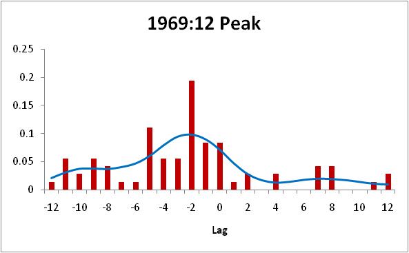 |
Although for this episode the “date-then-aggregate” approach would assign a date a little earlier than the historical turning point, for most of the postwar recessions it is remarkable how similar the dates are to the traditional designations. Interestingly, when Stock and Watson applied their algorithm to a series for monthly real GDP that they have developed, they found that it would have designated the 1969 downturn as having begun 4 months earlier than the NBER 1969:M12 date. Watson attributed this to the possibility that the Zarnowitz and Moore dates were based in part on nominal indicators that had become less reliable given the accelerating inflation at the time.
| NBER date | peak or trough | Aggregate (using GDP) then date | Date then aggregate (using median) |
|---|---|---|---|
| 1960:M4 | peak | -1 | -2 |
| 1961:M2 | trough | -2 | 0 |
| 1969:M12 | peak | -4 | -2 |
| 1970:M11 | trough | 0 | 0 |
| 1973:M11 | peak | 0 | 2 |
| 1975:M3 | trough | 0 | 0 |
| 1980:M1 | peak | 0 | -1 |
| 1980:M7 | trough | -1 | 0 |
| 1981:M7 | peak | 0 | 0 |
| 1982:M11 | trough | -3 | 0 |
| 1990:M7 | peak | 0 | 0 |
| 1991:M3 | trough | 0 | 1 |
| 2001:M3 | peak | -3 | |
| 2001:M11 | trough | 1 | |
| 2007:M12 | peak | 6 | 0 |
There are a few other episodes where the procedures might have suggested minor changes from the NBER dates, most significant of which is the 2001 recession, which the behavior of individual series suggests might have started in December 2000, while the Bry-Boschan algorithm does not designate this as a recession at all based on Stock and Watson’s monthly GDP measure. But the surprising finding is how little difference there is among the three dating procedures. It seems to make little difference whether you view a recession as an aggregate event, or as a collection of problems simultaneously hitting individual sectors. You’d identify pretty much the same episodes arriving at about the same times with either perspective.
Once again, this work seems a bit over-quanted to me. I’d like to see a little more emphasis on causal relationships, a little less on databases and statistics packages.
Having said that, understanding the business cycle is a critically important for strategic business planning. A company’s capital structure–its debt/equity ratio and st/lt debt structure, as well as its contracting and hedging policy–is implicitly a function of beliefs about the business cycle and the probability, timing, depth and duration of the next recession. As a result, this topic lies at the very heart of investment banking and equity investing.
And yet, it appears to me that the business community is largely in the dark on the topic. For example, Bear Stearns and Lehman Brothers were essentially victimized by the business cycle, or rather, by the unending optimism that there wouldn’t be one. I think the difference with Goldman Sachs was that the Goldman understood that no one lives forever. It employs a huge number of incredibly smart people, and apparently, management listens to them.
In any event, it would be useful to drag a few economists out of statistics-land to do some real world consulting on the topic, that is, conducting analysis primarily in terms of decision variables faced managers and policy-makers.
Did you see the articles in the May 2010 AER discussing the business cycle? (Sinai, etc.)
If you did, what did you think of them?
Economics is a science. The problem is that there aren’t any scientists.
Any intuition on why I see no blue in that figure? I see green, yellow, various shades of red, but the blue area (which seems to be a business ‘boom’) is not represented. Or is it just ‘blended’ in? (Or is my monitor just that bad?)
Interestingly, many of the presenters have UCSD ties. In additon to UCSD professors Hamilton and Timmermann, both Mark Watson and Tim Bollerslev were UCSD PhD recipients.