The exchange between Brad Delong and Greg Mankiw ([1] [2], followed up by [3] [4]) reminded me of some earlier work I’d done with Yin-Wong Cheung on the time series properties of real GDP, back in the “unit root” wars. Briefly, Mankiw was alluding to work with Campbell indicating GDP was well approximated as an ARIMA process, while Delong is arguing that using unemployment, which is trend stationary, indicates that indeed sharper increases in unemployment presage more rapid GDP growth. The former characterization is univariate in nature and the latter is bivariate. Of course, we’ve moved on since those days — the entire VAR and SVAR literature expands the set of variables, but at the cost of greater complexity — but simple characterizations can still be useful.
This brings me to the results Cheung and I obtained. In “Further Investigation of the Uncertain Unit Root in U.S. GDP” (NBER technical working paper here), we found that using post-War quarterly GDP up to 1994, we couldn’t reject the null hypothesis of a unit root, nor the null hypothesis of trend stationarity (using the ADF and KPSS tests, respectively). However, for annual data from 1869 to 1994, we could reject the unit root null and fail to reject the trend stationary null (we were working with per capita numbers, but the difference is unessential).
Here’s a plot of (log) GDP.
Figure 1: Log US GDP in Ch.2000$, SAAR. NBER defined recession dates shaded gray. Assumes current recession has not ended by 2008Q4. Source: BEA GDP release of 27 February 2009, and NBER.
I thought if I updated the analysis to include data up to 2008, I’d obtain similar results. Imagine my surprise when I found that for data 1967q1-2008q4, the ADF (w/constant, trend) test rejects the unit root null with a p-value of 0.048, and the Elliott-Rothenberg-Stock Dickey-Fuller test at the 0.01 level. At the same, the KPSS (trend stationary null) test fails to reject at conventional levels. (The annual results confirm the results Cheung and I obtained earlier). In other words, over the last forty years, log US GDP looks trend stationary.
What’s the relevance of these findings to the current debate? First, let me say I don’t think this has any impact on how one thinks about the relative importance of technology versus demand shocks. Second, I don’t think univariate analyses are the only way to go (for instance, in ordinary times, one might want to use consumption to infer potential GDP, and hence identify the trend in GDP). But what it does tell me is that the Campbell-Mankiw characterization of real GDP as being best fit by an ARIMA is perhaps no longer most apt. (For more on unit roots and trends from a nontechnical perspective, see this post.)
Two caveats.
- Just because one finds the data rejects a TS null doesn’t mean that that is the best way to treat the data in, say, regressions involving other variables. I.e., just because the data is trend stationary doesn’t mean that shocks to the series can’t be persistent. They might be so persistent that a unit root characterization is not a bad approximation.
- The rejection of the unit root null is sample dependent. Extending the sample back to 1947q1 yields a failure to reject the unit root null (the series still fails to reject the trend stationary null).
A simple regression of log GDP on a time trend and lagged log GDP, over the 1967q1-08q4 period yields the following:
yt = 0.424+0.0004time + 0.945yt-1
Where Adj-R2 = 0.9995, SER = 0.008
The AR1 coefficient of 0.945 (se = 0.03) implies a half life of 12.25 quarters, or slightly over 3 years for a deviation from output. Since AR coefficients are biased downward, this is a downwardly biased estimate of the half life.
Given that output is trending upwards (at about 3% per annum, in log terms) in a deterministic fashion, then the argument that big drops in output are accompanied by faster growth rates makes sense. The CEA post that makes use of the regression from the 2009 Economic Report of the President [large pdf] produced by the Bush White House (reproduced below) is in this world appropriate (in Mankiw’s unit root world, it wouldn’t be appropriate).
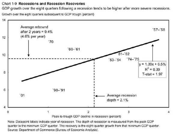
Chart 1-9: From Economic Report of the President, 2009 Chapter 1 pdf.
That being said, I think that additional information is always useful. And in this case, I stressed (in my last discussion of this graph) that the overpredicted growth rates were for the recoveries associated with financial system problems, such as a credit crunch. This means (in my opinion) that it is essential to fix the banking system in order for the faster growth to be realized.
Note that I haven’t addressed any issues regarding trend breaks as an alternative to unit roots or trends. Interested readers can refer to this paper, in a cross-country context.
Update, 7:50am Pacific 3/5: Steve Blough reminds me of another caveat: “Just because a time series has a unit root doesn’t mean there isn’t a substantial “bounceback” (mean reverting) component. In a univariate model ARIMA model that just means a large negative dominant moving average root. The mere presence or absence of a unit root doesn’t mean much of anything about persistence over a finite horizon.”
Dear Menzie
Interesting to see the amount of empirical analysis that participants have drawn on in this topic – compared to many of the macroeconomic debates which rely more on theoretical models. In the following (not especially technical) article I have tried to tease out some of the underlying theoretical assumptions which might lead to the unit-root or trend-stationary results:
http://www.knowingandmaking.com/2009/03/recession-and-recovery-krugman-and.html
Menzie: What lag length did you use for computing the ‘long-run variance’ for the KPSS test statistic and how did you select/identify it? KPSS (1992) suggest using a lag length such that the estimate of this long-run variance settles down. But exactly what empirically constitutes such ‘settling down’ can be rather ambiguous, and setting the lag length ‘too high’ can generate a considerable loss of ‘power.’ [Conversely, setting it ‘too low’ can generate substantial positive size distortion, as shown by Caner and Kilian (JIMF, 2001) and, several years earlier in a paper that never received much attention (no doubt because of the outlet in which it was published, after several ‘higher’ attempts), me (JMACRO, 1997).]
I’m glad that someone that understands the debate has finally pointed out that careful use of unit root tests lead to the conclusion that post-war US GDP does not look like it has a unit root.
But I think this also misses an important point; there is much clearer evidence to support the assumption of a strong post-recession bounce-back in output growth.
In my mind, the nicest exposition of this was in the Beaudry and Koop paper (JME 1993 “Do recessions permanently change output?” doi:10.1016/0304-3932(93)90042-E) Using very simple regressions, Beaudry and Koop demonstrate that recessions have quite different dynamics from other output shocks. As they state in their abstract, “…the effect of a recession on the forecast of output is found to be negligible after only eight to twelve quarters, while the effect of a positive shock is estimated to be persistent and amplified over time. Our results may therefore help reconcile two antagonistic views about the nature of business cycle fluctuations.”
While that article provides simple and clear evidence of the effect, the literature documenting it is much richer. I’ve commonly seen the idea refered to as Friedman’s “Plucking Hypothesis”; the idea being that when output is pulled down below potential by a recession, it quickly snaps back. Simon Potter (with and without coauthors) wrote several articles investigating and further documenting evidence of the nonlinearity in the dynamics of US output in the late 90s (e.g. Pesaran and Potter JEDC 1997, Potter JAE 1995.) We can also get asymmetric dynamics from a standard Hamilton-style Markov-switching model; since the recession state also tends to be less persistent state, we revert more quickly towards trend growth rates when we begin in a recession state than when we start in an expansion state. (I’m sure JDH can state this result with greater precision than I can and I’m surprised that he has not yet weighed in on this issue.)
Bottom line: I think the evidence to support the “strong bounce-back view” is much stronger than Mankiw makes out. I think this is because he restricts himself to the assumption of symmetric dynamics.
Thanks for the link Leigh, and good question about the lags, Rothman, good review all around from Menzie.
The possibility I conjecture is a collapse of some hierarchy of sectors, which would make the linear process appear to have fewer system variables (detectable above standard noise). A general model is a Kalman filter model, the significant system modes, summed in time, yields GDP which thus has the same number system variables in time. We need to be doing Karhunen-Love decomposition to see if we can find some significant changes.
But, if it is really a productivity shock meeting an artificial constraint, and ultimately means greater than trend productivity increases. But it is hard to detect for we are particularly at the non-stationary phase, meaning, the consumer changed his Kalman filter model in is head, and variances are high as he has fewer data points.
Ask how many goods “productions” does the consumer track in his normal life, and that number should be the number of system variables by an eigenfunction decomposition, and Mankiw is good at that.
But, I still think a long term spurt in productivity.
Since this recession is an off-the-chart 5% or larger decline in GDP, are we to expect the post-recession bounce-back to be more than 12% for the subsequent 2 years?
That WOULD be necessary just to get back to the ‘potential GDP’ line from the CBOE, which we currently are very far from.
I noticed that Brad did not include an explicit specification of the bivariate model. Is there a simple, canonical bivariate VAR that you prefer for modeling the types of dynamics here, and do you agree with several of the commenters here than the dynamics are actually properly modeled as non-linear?
P.S. great post for those of us learning – one gets to see the mechanics underlying the debate!
From article [1] above — ” a key fact is that recessions are followed by rebounds. Indeed, if periods of lower-than-normal growth were not followed by periods of higher-than-normal growth, the unemployment rate would never return to normal.”
I would argue that proposed government (permanent) intervention in health, energy, financial markets, others?, will decrease efficiency within the U.S. economy. The result could be a higher equilibrium level of unemployment. If true, then output and output growth need not return to their prior trend levels. Thus, the much anticipated bounce it gdp growth may be less than expected.
In other words, if you think Obama’s policies will move us closer to a Eurpoean model then we should expect a lower trend growth rate and a higher trend unemployment rate.
Just a… phillosophy of statistics question, for those of you more versed in stats:
Why would you automatically reject a null hypothesis that is p=0.048?
I wouldn’t treat it the way I would treat one that is 0.0048, that’s for sure (nor would I treat it like one that is 0.48).
That’s a gray area statistically, don’t you think? 95% confidence is ultimately a convention, not a law of the universe, right?
Hi Menzie – Please add to your caveats “just because a time series has a unit root doesn’t mean there isn’t a substantial “bounceback” (mean reverting) component. In a univariate model ARIMA model that just means a large negative dominant moving average root. The mere presence or absense of a unit root doesn’t mean much of anything about persistence over a finite horizon.
Thanks to all for the for the excellent comments!
Phil Rothman: Good question – the automatic bandwith selection option in Eviews selected 9 lags (Newey-West with Bartlett window). I manually tried smaller and larger lag lengths with the results unchanged.
GK: If you’re looking at the ERP2009 graph, well, GDP has only decline about 2.7% relative to GDP peak so far. Let’s assume that the total decline is 5% as you posit, then yes, the regression line implies something like 12% growth over two years, or 6% growth each of two years, on average. Of course, the confidence bands expand as one gets to the extreme values of the X axis…
SvN: Yes, I agree that I’ve compared the simplest of specifications, and lots of nonlinearities (threshold effects, asymmetries) are possible. Thanks for these references.
tj: Plausible. Kind of depends on what you think the regulation will be on (maybe more regulation of finance results in more sustainable growth, with less boom/bust behavior…) and what the stimulus funds will be spent on (Think “Federal highway system” in the 1950s).
Steve Blough: Thanks for catching that. I was mired in an AR world, and your comment highlights the difficulties in not only discerning whether there are deterministic or stochastic trends, but also appropriate time series model, when one differing ARIMA models are very close in terms of goodness of fit.
But I thought the whole theme of many of the comments recently is that all trendlines have been permanently revised down, and we cannot simply ‘return to the trendline’.
I think we can, which is why we eventually have to have a year, maybe even two, of 6%+ GDP growth just to get back to potential GDP. This is what happened in 1983, where GDP growth was 7.2%.
Regarding the discussion about recovery after crises, there is a paper by Cerra and Saxena in the march 2009 issue of the American Economic Review, in which they point out that losses due to financial crises seem to have a permanent effect on output. So how would this result be affected by the characterisation of output as being trend stationary or difference stationary?
Francisco Villareal: Don’t take anyof the results as gospel. Power for all these tests is probably low. Empirical size…well Cheung and I tried to address this in our JBES paper, but I haven’t here. In any case, Cerra and Saxena’s findings are consistent with my observation that recoveries from the 1990-91 and 2001 recessions (that have a financial stress component) are overpredicted by the regression in Chart 1-9 from ERP2009.
While I think the Cerra and Saxena results are interesting, I would caution inferring too much regarding the time series characteristics of real GDP measured in constant international dollars across a broad set of countries, because of the results Cheung and I obtained in our Oxford Economic Papers article.
Menzie-
Thanks for posting the Delong/Mankiw debate and your comments on “Unit Root” and “Trend Stationary” behavior. Being a neophyte to econometric literature, I was unfamiliar with the terms.
I would make the following observation: The persistent increase in liquidity in the post-war period from 1946 to 2007 resulted in relentless inflationary pressures and consumer decisions to buy quickly before prices escalate further… In other words- Unit Root behavior. The current worldwide banking failure has resulted in rapid deflation and changed consumer behavior. With falling prices Trend Stationary logic is ascendant, with purchases delayed for a better price.
Perhaps its my Midwestern upbringing, but I am far more attracted to behavior that delays consumption until actual utility overtakes thriftiness. This conserves scarce resources and improves return on investment.
I’m convinced that the US government will only slowly work-out the finance/banking insolvency, and US households can only slowly pay-down their credit leverage. This means that we can expect a fairly protracted period of declining or stagnant liquidity. Trend Stationary behavior will likely persist, and the rebound from this recession will likely be slow. A very good thing if we are interested in correcting the pathology that got us into this crisis in the first place.
I would stress that the amount of snap-back growth we get following a downturn is not a mechanical function (even if we allow the function to be nonlinear) of the magnitude of the downturn. My view is that the amount of snap-back growth we get is stochastic, so the permanent output loss associated with this recession is an estimate that we will have to revise as we learn more about how much snap-back growth is realized.
Dueker (2006) illustrates this view with a four-state Markov model of GDP. It shows how the expected output loss associated with a recession evolves across time and compares it with an HP output gap.
words of some important economists (Harvard, Yale etc) related to the last major downturn and prospects for a Growth Bounceback can be found here :
http://www.ritholtz.com/blog/2006/11/1927-1933-chart-of-pompous-prognosticators/
well menzie and folks around, what do we really learn from this :
1) cit. MDueker: ..the amount of snap-back growth we get following a downturn is not a mechanical function.
2) cit. MDueker:.. snap-back growth we get is stochastic.
3) Never trust old men, they have nothing to loose.
That’s rather amusing John Lee. Nice to see Keynes and Fisher in the list of Pompous Prognosticators.
We have empirical evidence that the forecasting abilities of most economic models are close to zero with the qualified exception of the yield curve model.
Do we have any studies of the forecasting abilities of smart people versus dumb people, well-educated people versus not so well-educated people, numerate versus innumerate?
Or do smart, well-educated, successful people simply get called upon to make public forecasts more often than others? That would be a variation on the theme that people want to know what an informed, competent person “knows” not what that they understand what they do not know. Translation: certainty sells.
By implication, either potential GDP must be revised down as a result of a recession, or at some point there must be catch-up growth in excess of historical averages.
Keep in mind, all this is backward-looking technical anaylsis. If you used the same methodology, you would have concluded that ‘housing prices never go down’ in 2006. A cursory look at the Case-Shiller index would have strongly suggested otherwise.
In my opinion, this recession is about the inability of the global economic system to accommodate the growth of China. On the financial level, excess liquidity from China’s growth blew out the US financial system. On the commodity side, China’s demand blew out the commodity supply system, including for oil, coal, iron ore, copper, etc.
Or put another way, this recession is in large part about the US migrating from being a large open economy to being a small open economy. Let’s see some forward-looking analysis on that. That should tell us more about the shape of the recovery.
“In my opinion, this recession is about the inability of the global economic system to accommodate the growth of China. ”
I don’t agree. Why now, rather than at any other time in the last 30 years?
And if China is still growing so fast and is so big, would it not keep the global economy out of recession?
Furthermore, this would cause rapid technological innovation in order to find solutions for China in energy, materials, telecom, etc.
The linear regression in Chart 1-9 is mis-specified. Do the math. They screwed it up.
The peak-to-trough declines for the 1970 and 2001 recessions are incorrect.
Conjure Bag says, “Have a nice day.”
What would the result be if this type of analysis was applied to Japan? It might give some insight to the magniture which a broken credit system retards normal mean reverting behavior.
magniture = magnitude.
mp: Hard to tell what you mean; I assume you don’t mean mis-specified in the sense you know the true model and it’s different than the one Ed Lazear and the CEA used. Is it the calculation of peak-to-trough, and hence the observation point for the 1970 and 2001 recessions? Note the footnote indicates they are not using NBER defined peaks and troughs.
“It might give some insight to the magniture which a broken credit system retards normal mean reverting behavior.”
I think the global economy reverts to the mean rather quickly (and even in the GD, it did so relatively fast). But individual countries can lag permanently. Much like a stock that continues to lag the S&P500 for a long time.
So the global economy can mean-revert even if the US does not. Of course, the slack would have to be picked up by a supercharged growth rate in emerging Asia.
“I assume you don’t mean mis-specified in the sense you know the true model and it’s different than the one Ed Lazear and the CEA used.”
Poor choice of words on my part.
“Note the footnote indicates they are not using NBER defined peaks and troughs.”
I’m aware of that. Using their methodology, I agree with every one of their peak-to-trough declines except two: the one in 1970 and the one in 2001. The difference is material to the final equation, correlation coefficient and t-statistic.
Note also that “Average Annual Growth Rate in Subsequent 8 Quarters,” identified as Table 2 on the White House web site, is actually the *annual* compound rate necessary to yield the 8-quarter growth spurt. They didn’t compound on a quarterly basis. This may be a minor point to some, but in a $12 trillion economy it would seem to me that one-tenth of a percent matters.
Conjure Bag says, “Hi, Professor!”
Before leaving, I would like to add one final comment re the “growth spurt.”
I think Feldstein is right. The wealth effect on households from the decline in house prices and the declining stock market has blown an enormous hole in GDP going forward. We’re probably talking $500 billion, at least until the wealth comes back.
I wish President Obama and his administration all the best but, if they really think their stimulus is going to reach the streets–to fill that hole–in time to have a meaningful impact on H2, they’re deluding themselves.
“They didn’t compound on a quarterly basis. This may be a minor point to some, but in a $12 trillion economy it would seem to me that one-tenth of a percent matters.”
Seriously, mp? You figure we should string them up for not publishing a $100B smaller GDP stat? You read the 11 digit GDP stat because….you are fond of large numbers?
Do you think that the compilation of this stat or any of its components, is anywhere close to a tenth of a percent accurate?
If I were to ask you how much you weighed, would you give the hourly record so that we could tabulate it to within 0.1%?
Good to see you make it off the CR board sometimes.
Regards to you, Calmo!
This was a great post because it:
1) Discussed a current news topic related to economics
2) related it to acedemic research
3) included original research on economic data that we could replicate on our own.
There was an article in the WSJ that related to this topic on hysteresis of the unemployment rate.
http://online.wsj.com/article/SB123654666022864641.html
Question, has anyone applied this analysis to Japan over the last 25 years?