My latest research paper reviews efforts to supplement the declarations by the National Bureau of Economic Research as to the beginning and ending of economic recessions with determinations made by purely mechanical algorithms.

From the paper’s abstract:

This paper surveys efforts to automate the dating of business cycle turning points. Doing this on a real time, out-of-sample basis is a bigger challenge than many academics might presume due to factors such as data revisions and changes in economic relationships over time. The paper stresses the value of both simulated real-time analysis– looking at what the inference of a proposed model would have been using data as they were actually released at the time– and actual real-time analysis, in which a researcher stakes his or her reputation on publicly using the model to generate out-of-sample, real-time predictions. The immediate publication capabilities of the internet make the latter a realistic option for researchers today, and many are taking advantage of it. The paper reviews a number of approaches to dating business cycle turning points and emphasizes the fundamental trade-off between parsimony– trying to keep the model as simple and robust as possible– and making full use of available information.

The paper discusses several reasons why such efforts might be of interest. Here’s one:

A second benefit of a purely objective algorithm for making these determinations in real time is that it would ensure that the process is completely apolitical. Although no one has accused the NBER of altering its announcements on the basis of political considerations, the pressure is undeniably present to delay the announcement that a recession has begun or accelerate the announcement that a recovery has begun if one’s goal were to help the incumbent. In the October 13, 1992 debates, then vice-presidential-candidate Al Gore referred to the “worst economic performance since the Great Depression.” Although the recession of 1990-91 is now seen as one of the shortest and mildest of the postwar recessions, it was not until December 22, 1992– after the presidential elections– that the NBER announced that the recession had actually ended in March of 1991. If it had been the case that the recession that began in August 1990 was still ongoing as of October 1992, Gore’s statement would have factual support in the sense that the ongoing recession would have been the longest on record since 1933. Being able to issue these announcements on the basis of a pre-determined, purely mechanical algorithm would insulate the procedure from any possible charges of partisanship.

For the last five years, I have been using Econbrowser as a forum for publicly reporting the real-time output of a mechanical GDP-based algorithm for dating U.S. business cycle turning points. The graph below plots those inferences in the form of our GDP-based recession indicator index. Values to the left of the vertical line are what I referred to above as “simulated real time”– each observation plotted was constructed solely from a vintage data set as it would have been reported at the indicated date. To the right of the vertical line are “actual real time” numbers– each observation plotted was publicly announced at the indicated date.

Graph plots for each quarter t the value for Prob(S_t|Y_t+1) where Y_t+1 is the history of observed GDP growth rates as reported as of date t+1.

Based on the procedure detailed in my 2005 paper with Marcelle Chauvet, the algorithm determined that the most recent recession began in the fourth quarter of 2007 and ended in the second quarter of 2009. A subsequent economic downturn would be viewed by this procedure as the beginning of a new recession rather than a continuation of the previous recession. Here is the simulated real time and actual real time record of the algorithm.

My new paper also reviews the performance of a number of alternative algorithms. Marcelle Chauvet and Jeremy Piger (2008) suggested an approach that uses growth rates of industrial production, personal income, sales, and employment. Professor Piger has been regularly updating these inferences on his web page since August 2006. There is a trade-off in these methods between trying to make an inference using the most recent available data about where the economy is at the moment (called the “filter probabilities”), or waiting for data to be revised and the trend to become clearer before trying to form an inference about where the economy was n months previously (called the “n-month smoothed probabilities”).
Piger’s actual real-time filter probabilities for each month are plotted in the top panel of the figure below. This series first moved above 50% in Piger’s November 1, 2008 report which was based on data describing August. The probability moved to 99.2% when the September data became available but fell back to 16.1% with the next month’s data which showed industrial production and real personal income less transfers to be growing again in October. Chauvet and Piger (2008) had recommended an inference rule of declaring a recession as soon as three consecutive values of recent smoothed probabilities were all above 80%. This threshold was passed with the release of the October data, for although the current month filter inference was only 16.1% based on t= October 2008 data, the 1-, 2-, and 3-month smoothed probabilities at that time were still all above 80% (see the bottom panel of the figure below). Chauvet and Piger’s (2008) announced rule would then date the start of the recession as the earliest n for which the smoothed probability was above 50%, which turned out to be February 2008. Thus their approach would have announced on January 1, 2009 that a recession had started in February 2008, although the filter probabilities available in January 2009 raised the possibility that the recession could already have been over by October. Subsequent data confirmed the downturn was ongoing (panels 2 and 3 of the figure). The Chauvet-Piger rule of waiting for a reading of 3 consecutive months below 20% would have resulted in a declaration in January 2010 that a recovery likely began in July of 2009.

Source: reproduced from Hamilton (2010); constructed from data supplied by Jeremy Piger.

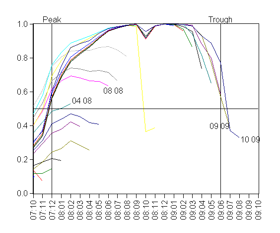
My 2005 paper with Chauvet proposed a similar 4-indicator inference. One important difference from the specification of Chauvet and Piger is the reliance on the BLS household survey for the measure of employment rather than the establishment payroll data. The figure below shows the sequence of smoothed probabilities associated with different vintages of data. This model would have sent a signal in August 2008 that a recession had begun in December 2007. Like Piger’s calculations, it showed a temporary hope of an end when only data through October 2008 were available. Chauvet used this model to announce on her website in October of 2009 that the recession ended in June or July of 2009.

Source: Marcelle Chauvet.

One of the most promising approaches reviewed in my paper is that developed by

Camacho, Perez-Quiros, and Poncela (2010). They show how one can use an unbalanced panel of mixed-frequency indicators to update an inference daily as each new datum gets released. The figure below reports the probabilities of a Euro-area recession that would have been calculated by their approach based on the actual data available as of each day during 2008 and 2009. The model yields a remarkably sharp and stable inference over this period, with the probability jumping from 3.8% on June 24, 2008 to 98.1% by July 24, 2008. The probability remained above 69% until April 23, 2009, at which point it fell to 6%.

Source:
Camacho, Perez-Quiros, and Poncela (2010).