I’m just back from a two day conference at the Norges Bank‘s conference center in the mountains north of Oslo (organized by Karsten Gerdrup, Christian Kascha, Francesco Ravazzolo and Dagfinn Rime). For me as an end-user of econometric methods, this was a great experience. I got to see some recent developments in applying time series methods to problems in macro and finance (and to see Norway for the first time). Here were some of the papers presented and discussed (I’ve omitted the papers that are not posted online).
- Evidence on the Predictability of Oil Prices for US GDP, by Philip Rothman, East Carolina University, and Francesco Ravazzolo, Norges Bank. Discussant: Vincent Labhard, European Central Bank
- Factor Model Forecasts of Exchange rates, by Kenneth West, University of Wisconsin, with Charles Engel (UW) and Nelson Mark (Notre Dame). Discussant: Hilde Bjørnland, Norwegian Business School
- Optimal Forecasting of Noncausal Autoregressive Time Series, by Markku Lanne, Helsinki University, with Luoto (Helsinki) and Saikkonen (Helsinki). Discussant: Anders Rygh Swensen, University of Oslo.
- Stock market Liquidity and the Business Cycle, by Bernt Arne Ødegaard, University of Stavanger, Naes (Ministry of Trade and Industry) and Skjeltorp (Norges Bank). Discussant: Francesco Ravazzolo, Norges Bank
- Measuring Output Gap Uncertainty, by Shaun Vahey, Australian National University, Garrett (Birkbeck) and Mitchell (NIESR). Discussant: Knut Are Aastveit, Norges Bank
- Strongly Dependent Processes and Long Memory [1] [2], by Richard Baillie, Michigan State University, and Kapatanios (Queen Mary, London). Discussant: Nii Ayi Armah, Bank of Canada.
- Prior Selection for Vector Autoregressions, by Giorgio Primiceri, Northwestern University, Giannone (Free University, Brussels) and Lenza (ECB). Discussant: Gernot Doppelhofer, Norwegian School of Economics and Business Administration.
- The Predictive Power of the Yield Curve across Countries and Time, by Kavan Kucko, Federal Reserve Board, and Menzie Chinn, University of Wisconsin-Madison, Discussant: Christian Kascha, Norges Bank
All of the papers have substantive implications for the implementation of macroeconometrics, particularly going beyond the simple OLS regressions that I typically discuss on Econbrowser, but I’ll only discuss some of the papers that have some direct links to some of the recent policy/empirical debates.
The conference started with the paper written by Philip Rothman and Francesco Ravazzolo.
We study the real-time Granger-causal relationship between crude oil prices and US GDP growth
through an out-of-sample (OOS) forecasting exercise; we do so after providing strong evidence of
in-sample (IS) predictability from oil prices to GDP. Comparing our benchmark model without
oil” against those with oil” by way of both point and density forecasts, we find strong evidence
in favor of OOS predictability from oil prices to GDP via our point forecast comparisons when
we adjust our MSPEs to account for noise introduced under the null hypothesis that the parsimonious benchmark is the true data generating process. These results are consistent with
well-known IS results covering part of our OOS period, and also suggest that, in the 1990s and
2000s, oil prices have had greater predictive content for GDP than in the mid to late 1980s. By
way of density forecast OOS comparisons, while we do not find statistically significant evidence
of such predictability from oil prices to GDP for the full 1970-2008 OOS period, our results qualitatively also suggest substantial time variation in this relationship; predictability from 1970 to
1985, and increasing predictability near the onset of the Great Recession.
The research of Jim Hamilton came up a lot (no surprise); see for some context these posts: [3] [4] [5]. Lutz Kilian’s work also came up; see Jim’s take on his work here and here.
Ken West’s paper (with Charles Engel and Nelson Mark) was of great interest to me, given my research area:
We construct factors from a cross section of exchange rates and use the idiosyncratic deviations from the factors to forecast. In a stylized data generating process, we show that such forecasts can be effective even if there is essentially no serial correlation in the univariate exchange rate processes. We apply the technique to a panel of bilateral U.S. dollar rates against 17 OECD countries. We forecast using factors, and using factors combined with any of fundamentals suggested by Taylor rule, monetary and purchasing power parity (PPP) models. For long horizon (8 and 12 quarter) forecasts, we tend to improve on the forecast of a “no change” benchmark in the late (1999-2007) but not early (1987-1998) parts of our
sample.
Their Figure 1 depicts the three factors they identify.
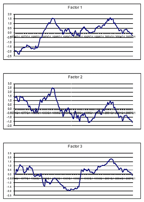
Figure 1 from Engel, Mark and West.
I find the results particularly interesting because of the finding that out-of-sample forecasting is more successful (vis a vis the random walk benchmark) at the long horizon, something which I had a hard time verifying in my work with Cheung and Fujii (which in turn was trying to validate the earlier results in Chinn and Meese (JIE, 1995) and Mark (AER, 1995).
Professor West noted that their model is just about on target for the June 2010 value of the dollar/euro exchange rate (not in the paper).
Bernt Arne Ødegaard’s paper (with Naes and Skjeltorp) observes:
In the recent financial crisis we saw the liquidity in the stock market drying up as a
precursor to the crisis in the real economy. We show that such effects are not new, in fact
we find a strong relation between stock market liquidity and the business cycle. We also
show that the portfolio compositions of investors change with the business cycle and that
investor participation is related to market liquidity. This suggests that systematic liquidity
variation is related to a flight to quality” during economic downturns. Overall, our results
provide an new explanation for the observed commonality in liquidity.
In particular, the authors find that the illiquidity ratio (ILR) is a particularly good measure predictor of subsequent economic activity. The ILR is measured as the absolute value of returns divided by volume.
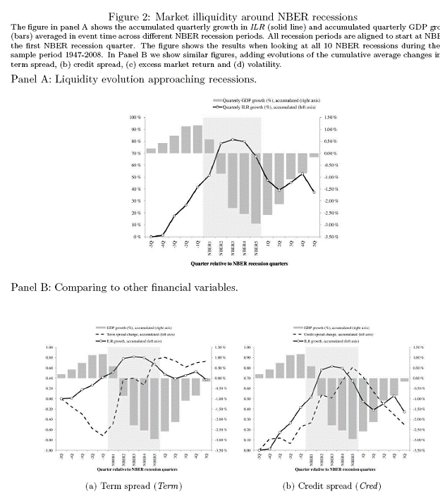
Excerpt from Figure 2 from Stock market Liquidity and the Business Cycle (forthcoming, J.Finance).
From Shaun Vahey’s paper (with Garrat and Mitchell):
We propose a methodology for producing density forecasts for the output
gap in real time using a large number of vector autoregessions in inflation
and output gap measures. Density combination utilizes a linear mixture of
experts framework to produce potentially non-Gaussian ensemble densities
for the unobserved output gap. In our application, we show that data revisions
alter substantially our probabilistic assessments of the output gap
using a variety of output gap measures derived from univariate detrending
filters. The resulting ensemble produces well-calibrated forecast densities for
US inflation in real time, in contrast to those from simple univariate autoregressions
which ignore the contribution of the output gap. Combining evidence
from both linear trends and more flexible univariate detrending filters
induces strong multi-modality in the predictive densities for the unobserved
output gap. The peaks associated with these two detrending methodologies
indicate output gaps of opposite sign for some observations, reflecting the
pervasive nature of model uncertainty in our US data.
The sensitivity of the estimates of the output gap to data revisions is illustrated in their Figure 2.
Figure 2 from Garratt, Mitchell and Vahey (2009).
Richard Baillie presented results from two papers. From Confidence Intervals For Impulse Response Weights From Strongly Dependent Processes”:
This paper considers the problem of estimating impulse response (IR)s from processes that are possibly strongly dependent and the related issue of constructing confidence intervals for the estimated IRs. We show that the parametric bootstrap is valid
under very weak conditions, including non Gaussianity for making inference on IR
from strongly dependent processes. Further, we propose, and justify theoretically, a
semi-parametric sieve bootstrap based on autoregressive approximations. We find that
the sieve bootstrap generally has very desirable properties and is shown to perform
extremely well in a detailed simulation study.
For me, the interesting results were the empirical ones pertaining to real exchange rates. They indicate high persistence (hard to obtain using standard autoregressive functions), and nonmonotonicity.
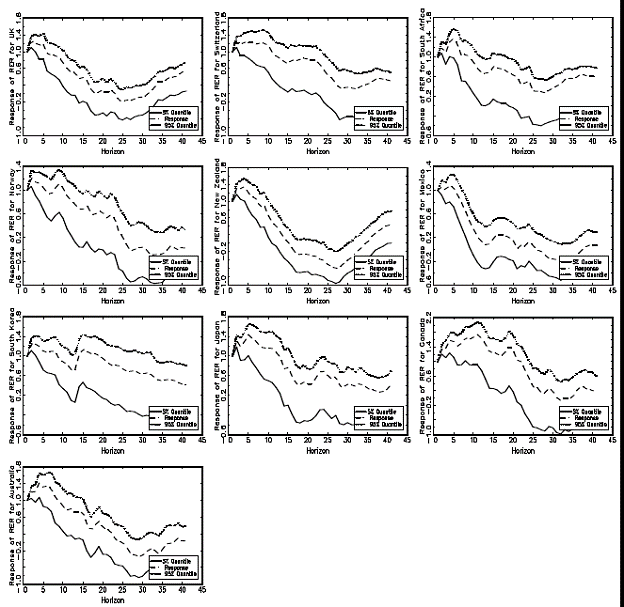
Figure 6 from Baillie and Kapatanios (2010).
I presented the final paper (coauthored with Kavan Kucko).
In recent years, there has been renewed interest in the yield curve (or alternatively,
the term premium) as a predictor of future economic activity. In this paper, we re‐examine the
evidence for this predictor, both for the United States, as well as European countries. We
examine the sensitivity of the results to the selection of countries, and time periods. We find
that the predictive power of the yield curve has deteriorated in recent years. However there is
reason to believe that European country models perform better than non‐European countries
when using more recent data. In addition, the yield curve proves to have predictive power even
after accounting for other leading indicators of economic activity.
An earlier version of this paper was discussed in this April 2009 blogpost. One thing I didn’t highlight in the earlier post is the fact that the yield curve coefficient becomes less statistically significant in some, but not all, countries in the later period. Figure 6 from the paper presents point estimates and 95% standard error bands for ten-year window rolling regression coefficients.
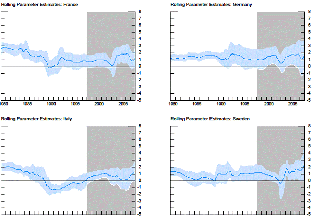
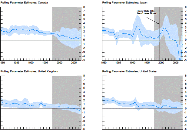
Figure 6 from Kucko and Chinn (2010).
The shaded area pertains to a period that some observers have tagged as evidencing reduced predictive power for the yield curve. Some of the speculation surrounds the “Great Moderation”, increased monetary policy credibility, and more recently the conundrum and the global saving glut. And for the European countries, the impact of the euro has been considered as a factor altering the yield curve link.
The discussant, Christian Kascha, provided some excellent insights into the paper. One point he makes is that one could compare the yield curve performance against a more comprehensive set of statistical models. He provides the following table:
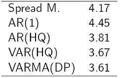
In other words, the spread does beat a AR(1), but not an AR selected by the Hannan-Quinn information criterion. Outperformance is even more marked when using multivariate models, such as a VAR and VARMA.
The day before the conference, there was a workshop on “Short-Term Forecasting in Central Banks”. The presentations are not available online, but Michael McCracken had an interesting paper “Forecast Disagreement among FOMC Members”.
Menzie: Thanks for the kind reference.
That all looks really interesting, unfortunately most of it went above my head. Can you recommend any resources for econometrics for dummies?
I would not dare to ask Pr Chinn to recommend any resources for dummies as he may ask which variable you want to integrate as dummy.
Meanwhile it is enjoyable to read Forecast Disagreement among FOMC Members”.
Was it Roosevelt or K Arrow whom said 10 yes and 1 no,the no caries over?
Menzie,
Thanks for the interesting summaries. So, with regard to the West and Engel paper that seems to go against your recent findings, while perhaps fitting in a bit more with some of Engels’ earlier work with Jim Hamilton (who deferred to you here on this matter), does this mean that we can beat the random walk in forex markets? More particularly, are the three factors each dominated by a partcular variable, or are they just effectively arbitrary, but orthogonal, combinations of the selected variables not amenable to any meaningful interpretation beyond plugging them into a computer and calculating?
Phil Rothman: You’re very welcome. This should be a paper that gets lots of attention.
James: I learned a lot from Granger, C. W. J. and Newbold, P. (1977). Forecasting Economic Time Series. Academic Press; second edition: 1986. I used to assign Walter Enders, Applied Econometric Time-Series, New York: John Wiley and Sons in my master’s level course in applied econometrics. Then of course, there is Jim Hamilton’s Time Series Analysis.
Barkley Rosser: The outperformance of a random walk has to be interpreted in the context of the analyst’s objectives. If one is interested in evaluating the economic model against a naive random walk model, the Clark-West model accounts for the estimation error that is associated with implementing the economic model (while that estimation error is absent in the random walk characterization). On the other hand, it is still true that the random walk will outperform the estimated models if all one cares about is which characterization fits best out-of-sample (i.e., is aiming to make money by way of having smallest RMSEs). For greater detail, see the Clark-West paper.
The factors are difficult to interpret. They are primarily statistical creations, although their importance for certain bilateral exchange rates is suggestive; so for instance the first pinciple component could be construed as a sort of euro area factor.