Today we are fortunate to present a guest post written by Michele Ca’ Zorzi (ECB) and Michal Rubaszek (SGH Warsaw School of Economics). The views expressed are those of the authors and do not necessarily reflect those of the ECB.

We have just released a new ECB Working Paper entitled “Exchange rate forecasting on a napkin”. The title highlights our desire to go back to basics on the topic of exchange rate forecasting, after a work-intensive attempt to beat the random walk (RW) with sophisticated structural models (“Exchange rate forecasting with DSGE models,”).

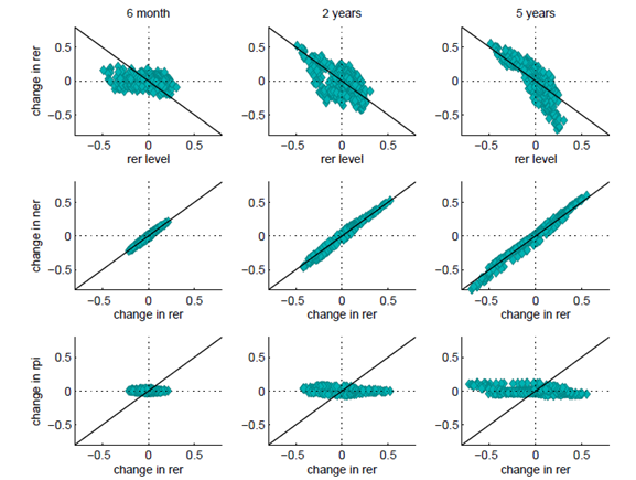
Cheung et al. (2017) have recently reaffirmed the difficulties of finding models that consistently outperform the RW; however they also concluded that the Purchasing Power Parity (PPP) model performs fairly well. The starting point of our analysis is an observation that in-sample there are two important regularities in foreign exchange markets in advanced countries with flexible regimes. The first one is that real exchange rates are mean-reverting over the medium term, as implied by PPP theory. For the EUR-USD rate this is illustrated by the upper panel of Figure 1. The second regularity is that the whole adjustment takes place via the nominal exchange rate (NER, middle panel) and not via relative price indices (RPI, bottom panel). These results immediately prompt the question: why have researchers not exploited these robust features in the data to beat the RW?

Figure 1: Exchange rate regularities for the euro dollar. Notes: Changes for a variable Y over horizon H are expressed as Δyt,H = y_t-y_t-H, where y_t=log(Y_t). The rer level is equal to the deviation of rer_t-H from the sample mean rer-bar. See also Eichenbaum et al. (2017).

In the paper we evaluate several competing models that should be able to exploit the two above regularities to forecast nominal bilateral exchange rates of ten currencies against the US dollar. The winner of the forecasting horse race is a half-life (HL) model, which just assumes that the real exchange rate gradually returns to its sample mean and that relative price indices play no role in this adjustment. The key advantage of this approach is its simplicity. It can be easily implemented using the following formula:

where Δner_t+h,h = ner_t+h-ner_t is a percentage change in the nominal exchange rate over horizon h, rer-bar is the sample average and ρ is the pace of mean reversion. Consistently with the meta-analysis of Rogoff (1996), we assume that half of the adjustment in RER is achieved in 3 years. This means that, in the case of monthly data, ρ=0.981.

The approach is so simple that it can be implemented on a napkin in two steps. Step 1 consists in calculating the initial currency misalignment with an eyeball estimate of what is the distance between the real exchange rate and its sample mean. Step 2 consists in recalling that, according to the above formula, one tenth of required adjustment is achieved in the first six months, one fifth in one year, just over a third in two years and exactly half after 3 years.

In the paper we compare this simple approach to the RW, which serves as a benchmark, as well as to other models, in which the pace of mean reversion over horizon h is estimated with individual currency time series (direct forecast, DF model) or panel data (PDF model). The comparison of the forecasts is done using the Root Mean Squared Forecast Error (RMSFE), where the relative performance is tested with the Diebold-Mariano and Clark-West tests.

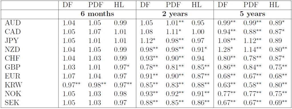
The results, which are presented in Table 1, show that the HL model beats overwhelmingly the RW at all horizons. Moreover, problems arise when attempting to carry out more sophisticated approaches, such as estimating the pace of mean reversion of the real exchange rate or forecasting relative inflation. Among the estimated approaches, in the paper we indicate that it strongly preferable to rely on direct rather than indirect forecasting methods. We also find that models estimated with panel data techniques (PDF) perform marginally better than those based on individual currency pairs (DF) but not enough to change the outcome. Even though both these models tend to beat the RW at horizons above 2 years, they tend to lose against the HL model, especially at shorter horizons.

Table 1: RMSFE for the NER with respect to the RW. Notes: The table shows the ratio of RMSFE from a given model in comparison to the RMSFE from a RW. Asterisks ** and * denote the 1% and 5% significance levels of the one-sided Diebold-Mariano (HL model) or Clark-West (DF and PDF models) with the alternative that a given model performs better than the RW.

Our findings have bittersweet implications. On the negative side, estimated models encounter a second formidable competitor that, like the RW, bypasses the estimation error problem. On the positive side the HL model is much more acceptable than the RW from the perspective of economic theory. Our analysis helps one to reconcile the evidence from different strands of the literature. The key takeaways are at least fourfold. First, PPP holds for advanced countries. Second, the nominal exchange rate is the driving force of the adjustment. Third, estimation error is the reason for failure of why many models do not outperform the RW, particularly at short horizons and with indirect forecasting techniques. Finally, the RW is beaten by a calibrated HL PPP model in a very robust and consistent way across a multitude of currency pairs.  

References

Ca’ Zorzi, M., M. Kolasa, M. Rubaszek, 2017. “Exchange rate forecasting with DSGE models”, Journal of International Economics 107 (C), 127-146.

Ca’ Zorzi, M., M. Rubaszek, 2018. “Exchange rate forecasting on a napkin”, ECB Working Paper No. 2151.

Cheung, Y.-W., Chinn, M. D., Pascual, A. G., Zhang, Y., 2017. Exchange rate prediction redux: new models, new data, new currencies, ECB WP No. 2018.

Eichenbaum, M., B. K. Johannsen, S. Rebelo, 2017. “Monetary policy and the predictability of nominal exchange rates”, NBER Working Papers 23158, National Bureau of Economic Research.

This post written by Michele Ca’ Zorzi and Michal Rubaszek.