The underlying data from which the U.S. unemployment rate and labor-force participation rate are calculated contain numerous inconsistencies– if one of the numbers economists use is correct, another must be wrong. I’ve recently completed a research paper with Hie Joo Ahn that summarizes these inconsistencies and proposes a reconciliation.
The data that everyone uses are based on a survey of selected addresses. An attempt is made to classify each adult living at that address as employed E, unemployed but actively looking for a job U, or not in the labor force N. The next month the surveyors try to contact the same address and ask the same questions. In any given month, some households are being asked the questions for the first time, others for the second time, and so on up to eight different rotation groups. The statistics for a given month come from summing the data obtained for that month across the eight different groups.
One of the well-known inconsistencies in these data is referred to in the literature as “rotation-group bias;” see Krueger, Mas, and Niu (2017) for a recent discussion. One would hope that in a given month, the numbers collected from different rotation groups should be telling the same story. But we find in fact that the numbers are vastly different. In our sample (July 2001 to April 2018), the average unemployment rate among those being interviewed for the first time is 6.8%, whereas the average unemployment rate for the eighth rotation is 5.9%. Even more dramatic is the rotation-group bias in the labor-force participation rate. This averages 66.0% for rotation 1 and 64.3% for rotation 8. Halpern-Manners and Warren (2012) suggested that admitting month after month that you’ve been continually trying to find a job but keep failing may carry some stigma, causing fewer people to admit to being unemployed in later rotation groups. Other respondents may believe they would be asked fewer or less onerous follow-up questions if they simply say they’re not actively looking for a job the next time they are asked.
Our solution is to model this feature of the data directly rather than sweep it under the rug. By studying how the answers across rotation groups differ systematically, we can translate the statistics for any given month into the answers that would have been given if they were based solely on people being interviewed for the jth time. For example, we model the tendency for people tend to be counted as N instead of U the more times they are contacted, and find that this tendency has increased over the sample. Our model allows us to calculate all statistics from the perspective of the answers that would be given by any given rotation group. We find that the answers people give the first time they are asked are easier to reconcile with other features we observe in the data, and the adjusted numbers reported below are based on the first-interview concept of unemployment.
A second problem in the data, originally noted by Abowd and Zellner (1986), is that observations are missing in a systematic way. The surveyors often find when they go back to a given household in February that some of the people for whom they collected data in January no longer live there or won’t answer. The standard approach is to base statistics for February only on the people for whom data is collected in February. But it turns out that people missing in February are more likely than the general population to have been unemployed in January. If the people dropped from the sample are more likely to be unemployed than those who are included, we would again underestimate the unemployment rate.
Our solution is to add a fourth possible labor-force status for each individual, classifying everyone as either employed E, unemployed U, not in the labor force N, or missing M. By combining this with our characterization of rotation-group bias, we develop the first-ever version of the underlying data set in which all the accounting identities that should hold between stocks and flows are exactly satisfied. By looking at what we observe about M individuals in the months when they are observed, we can adjust the data for the bias that comes from nonrandom missing observations.
A third inconsistency in the underlying data comes from comparing the reported labor-force status with how long people who are unemployed say they have been looking for a job. Consider for example people who were counted as N the previous month but this month are counted as U. The histogram below shows the percentage of these individuals who say they have been actively looking for work for an indicated number of weeks. Two-thirds of these people say they have been looking for 5 weeks or longer, even though the previous month they were counted as not in the labor force. Eight percent say they have been looking for one year, and another 8% say they have been looking for two years.
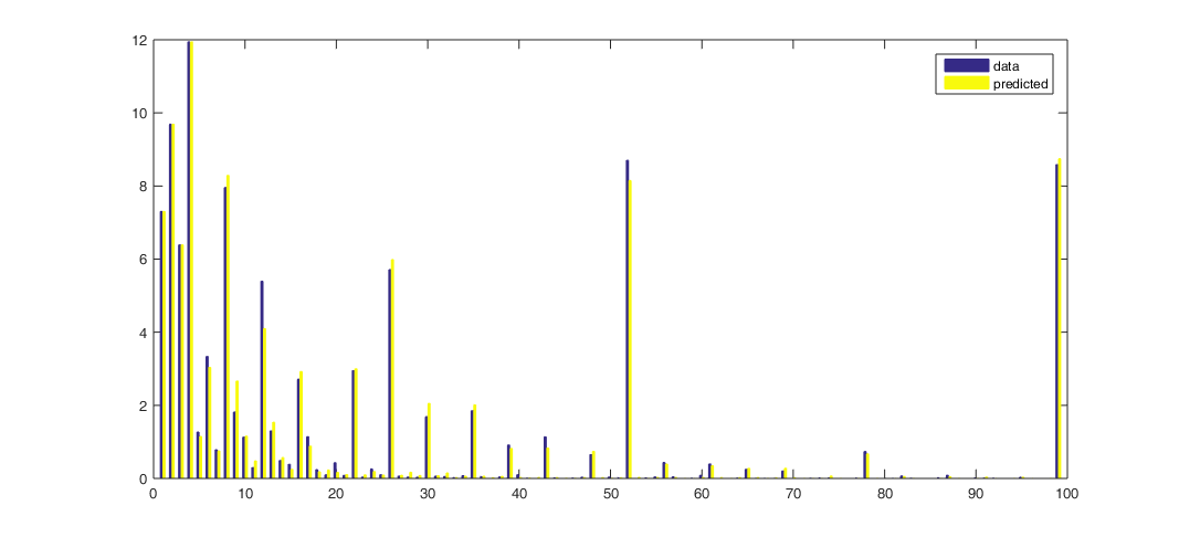
Horizontal axis: duration of unemployment spell in weeks. Vertical axis: of the individuals who were not in the labor force in rotation 1 and unemployed in rotation 2, the percent who reported having been searching for work at the time of rotation 2 for the indicated duration. Source: Ahn and Hamilton (2019).
A related inconsistency arises from what we observe the next month for individuals who are unemployed this month and say as of this month that they have been looking for six months or more. Far fewer of these individuals are counted as unemployed the following month than would be consistent with their reported unemployment durations. Either some of the labor-force designations are wrong, or people misreport how long they have been looking for work. In our analysis we conclude that both errors contribute to the published data.
One of the adjustments we make to reconcile these inconsistencies is to reclassify those individuals who report job search of 5 weeks or longer in the figure above as having been U rather than N the month before. We show that this also means that some of the individuals who are characterized as having “exited” long-term unemployment by becoming N should really be viewed as experiencing continuing spells of unemployment. In addition to the individuals’ own retrospective assessment at date t, we find that those people we reclassify from N to U have similar job-finding probabilities, and similar dependence of those job-finding probabilities on unemployment duration reported in month t, as do individuals who were classified by BLS as U rather than N in t – 1. Nearly half of those we reclassify from N to U at t – 1 were already characterized by BLS as “marginally attached to the labor force” in t -1 based on some of the other answers they gave in t – 1. Moreover, we find from the American Time Use Survey that many individuals who are N and not classified as marginally attached in fact spend as much time looking for a job as those classified as U.
A final issue with the underlying data can also be seen in the figure above– people seem to prefer to report some numbers more than others. On average, more people say they have been unemployed for 2 weeks instead of 1, and more people say they have been unemployed for 6 weeks instead of 5, even though in reality no one could be unemployed for 2 weeks if they weren’t first unemployed for 1 week. Our solution to this issue is to start with a coherent, smoothly decreasing representation of perceived durations and assume that people report those numbers with a particular form of censoring. Related approaches were taken by Baker (1992), Torelli and Trivellato (1993), and Ryu and Slottje (2000). Our approach differs from earlier studies in that we furthermore directly link data on stocks, flows, and durations. The numbers that our model predicts individuals would report are shown as the yellow bars in the figure above. We can describe the observed data very accurately.
The figure below gives one illustration of why all this matters. It considers a very fundamental question: if someone was unemployed last month, what is the probability that person will still be unemployed this month? Economists have used the data underlying the official statistics to answer this question in two different ways. One measure is based on number of people who are counted as unemployed in any given month. It calculates the number of people in the current month who say they have been unemployed for longer than one month as a fraction of the total number of people who were unemployed last month. This way of calculating the probability is plotted as the solid black line in the figure below. An alternative measure, based on labor-force flows, looks at the subset of individuals who were U last month and either E, N, or U this month. This measure calculates the number of UU continuations as a fraction of the sum UU + UE + UN. This flows-based measure is plotted as the dashed green line. If all magnitudes were measured accurately the two estimates should give the same answer. But in practice they are wildly different. The duration-based measure averages 70.7% over our sample, while the flows-based measure averages 53.7%. Our paper describes how the multiple problems mentioned above introduce biases into both of the measures, and develops the reconciled estimate shown in the dotted blue line.
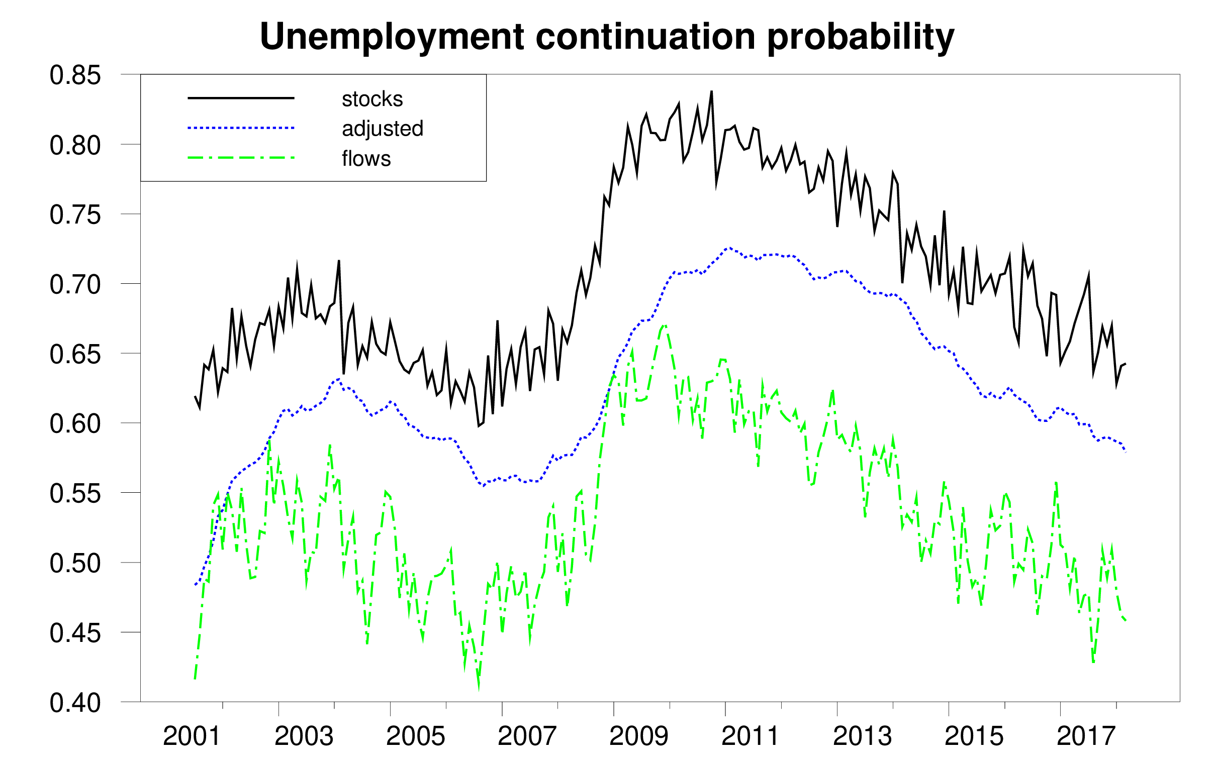
Probability that an unemployed individual will still be unemployed next month as calculated by: (1) ratio of unemployed with duration 5 weeks or greater in month t to total unemployed in t – 1 (solid black); (2) fraction of those unemployed in t – 1 who are still unemployed in t (dashed green); (3) reconciled estimate (dotted blue). Source: Ahn and Hamilton (2019).
We conclude that the true unemployment rate in the U.S. is 1.9% higher on average than the published estimates.
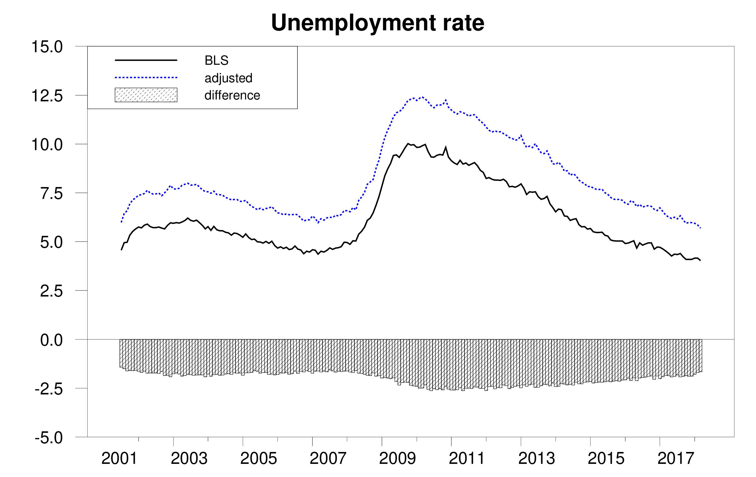
Unemployment rate as calculated by BLS (solid black), adjusted estimate (dotted blue), and difference (bars).
Source: Ahn and Hamilton (2019).
We also conclude that the Bureau of Labor Statistics has underestimated the labor-force participation rate by 2.2% on average and that the fall in participation has been slower than suggested by the BLS estimates.
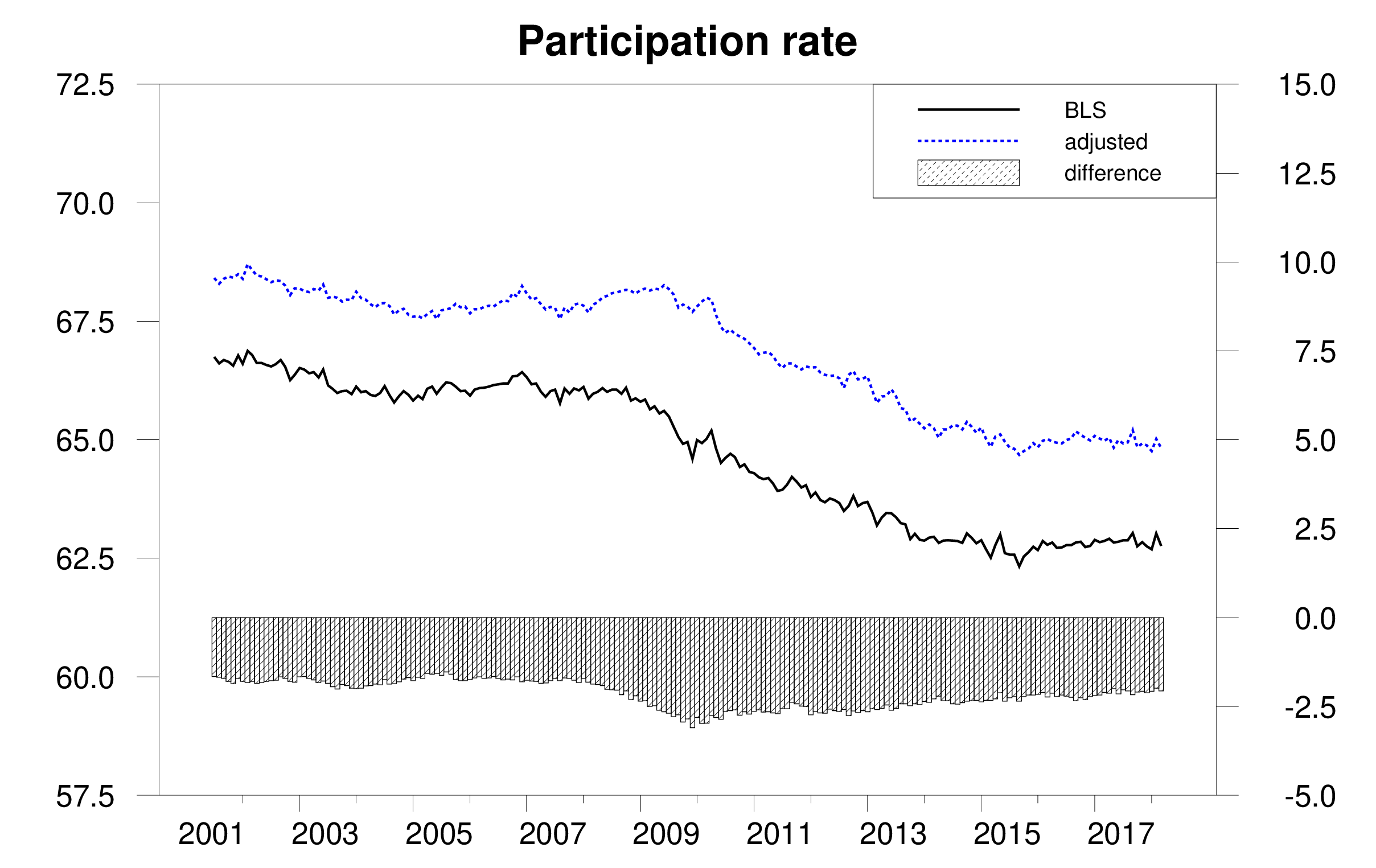
Labor-force participation rate as calculated by BLS (solid black), adjusted estimate (dotted blue), and difference (bars).
Source: Ahn and Hamilton (2019).
On the other hand, we find that reported average unemployment durations significantly overstate the average length of an uninterrupted spell of unemployment. A big factor in this appears to be the fact noticed by Kudlyak and Lange (2018) that some individuals include periods when they were briefly employed but nonetheless looking for a better job when they give an answer to how many weeks they have been actively looking for a job.

Average duration of unemployment in weeks as calculated by BLS (solid black), adjusted estimate (dotted blue), and difference (bars). Source: Ahn and Hamilton (2019).
Here is our paper’s conclusion:
The data underlying the CPS contain multiple internal inconsistencies. These include the facts that people’s answers change the more times they are asked the same question, stock estimates are inconsistent with flow estimates, missing observations are not random, reported unemployment durations are inconsistent with reported labor-force histories, and people prefer to report some numbers over others. Ours is the first paper to attempt a unified reconciliation of these issues. We conclude that the U.S. unemployment rate and labor-force continuation rates are higher than conventionally reported while the average duration of unemployment is considerably lower.
Wow!
Brad DeLong has more on the Moore nomination to the FED:
https://www.bradford-delong.com/2019/03/ha-ha-ha-ha-ha-larry-lindsey-and-john-taylor-please-please-appoint-us-to-something-there-is-no-plate-of-shit-so-large.html
Brad trashes a couple of Team Republicans for trashing what little reputation they ever had to endorse Moore. But read the article he links to as it is really stupid wet kiss to Moore as I noted in my two comments at Brad’s place.
I haven’t finished reading all of this yet, but I wanna say I am extremely glad you are quoting Alan Krueger in this blog post. I think he was a great man and I feel sorry I never got to meet him. Hope his family is being cared for. It’s hard to me to imagine the high-quality individual he was that Mr. Krueger didn’t “take some measures” along those lines, as regards his family’s safety and comfort, beforehand.
Many Christians believe there is only “one unforgivable sin”. That is the sin in which you cannot ask for forgiveness for, before you die. I like to think there are exceptions to this rule, and that there are some individuals such as comedian Robin Williams and Mr. Alan Krueger who shined so brightly, helped aid so many people in need, and gave joy to so many people, that exceptions are made. This is how I am choosing to think about it.
This is very interesting, your “missing M” almost becomes like an “error term” in an equation, yeah?? I mean not exactly like that, but “kinda”.
Here is a 2014 ungated version of the Krueger, Niu, Mas paper. It may be slightly different as it wouldn’t have the 2017 year updates to the paper.
https://www.princeton.edu/~amas/papers/RGB.August.pdf
If true would this partially explain the lack of real income gains among employees?
Also have you been able to break the numbers demographically among race, gender and age?
Let me elaborate: WOW!
There’s an awful of policy predicated on those numbers.
That makes a lot of sense the unemployment rate is 5.7% instead of 3.8% (in February 2019), for example, particularly with so many people moving out of California 🙂
Although, some are moving in (e.g. middle class outbound, out of desperation, and upper class inbound, although the recent tax law may increase frictional unemployment?).
So many dumb comments – so little time.
“particularly with so many people moving out of California”
YES!!!!!!!! PLEASE!!!!! PLEASE!!!!
STAY AWAY!!!!
California is full up and needs fewer people so rents and house prices will go down.
CA – nobody lives there anymore. It’s too crowded.
@ randomworker
Sometimes the best blog comments are the short ones. Our panel of judges says that’s 5-stars.
I’m assuming the BLS unemployment and participation graphs reflect seasonally adjusted data. How did your corrected data account for seasonality? What I’m getting at is whether or not there might be some seasonality component in the respondents’ perception of how they view their current status. It seems unlikely that a person’s self-perception of their employment status wouldn’t be affected by various seasonal factors; e.g., Xmas holidays, students arriving or leaving school, etc.
Also, this isn’t terribly important, but I was a little puzzled about the reference to modeling duration perceptions as an exponential distribution (page 13), but yet it looks like the data are discrete weeks. I’m assuming you used an exponential rather than a geometric distribution out of mathematical convenience. Not that it would make much practical difference I suppose.
2slugbaits: All the analysis was conducted using the raw seasonally unadjusted numbers. Seasonal adjustment is the very final step before producing the numbers in the last 4 graphs above. You’re right that predictions about weekly-clustered data are technically in the form of a geometric as opposed to an exponential distribution, though theoretical calculations can also be done using duration as if it is a continuous-valued variable. And you’re certainly right that this doesn’t make any difference for applications like this.
• An attempt is made to classify each adult living at that address as employed E, unemployed but actively looking for a job U, or not in the labor force N.
• A big factor in this appears to be the fact noticed by Kudlyak and Lange (2018) that some individuals include periods when they were briefly employed but nonetheless looking for a better job when they give an answer to how many weeks they have been actively looking for a job.
So, it seems that the employment rate E/(E+U+N+M) should be rather close to acceptable (perhaps a bit understated by those who include temporary employment as looking for a job) without a lot of manipulation whereas determining U versus N is the gray area. Has there been an attempt to look at an employment rate in this manner, knowing that it doesn’t address the issues of participation rate or unemployment rate?
I don’t pretend any expertise in this area, but it seems that if you can have one variable known with relatively high confidence that it could be a good measure of what is happening versus another measure (participation rate) that requires inferring what two other variables are. Not sure this is calculated the way I suggest, but if you look at the MAX year history, it seems to mirror the unemployment rate to a great extent (although I’d go with some smoothing… maybe three months). https://tradingeconomics.com/united-states/employment-rate
The unemployment rate is certainly an important indicator and even if understated give a relative measure of economic health. Perhaps by having information about N split into “not working and not looking for work” and “retired” the impact of demographic changes could be reduced and a better look at the “real” potential labor force be achieved. Does the survey attempt to account for these two groups? Of course, all of that still leaves the issue of “missing”.
Regardless, thanks for the insight into the complexity and limitations of the data. I appreciate the chance to learn.
Thanks for the well done study, JJm. It is especiially useful to have made the estimates about how these biases and errors have changed over time.
Moses might interested in what The Guardian is reporting on Stephen Moore and the issue of child support:
https://www.theguardian.com/us-news/2019/mar/30/trump-stephen-moore-federal-reserve-board
“Stephen Moore, the economics commentator chosen by Donald Trump for a seat on the Federal Reserve board, was found in contempt of court after failing to pay his ex-wife hundreds of thousands of dollars in alimony, child support and other debts. Court records in Virginia obtained by the Guardian show Moore, 59, was reprimanded by a judge in November 2012 for failing to pay Allison Moore more than $300,000 in spousal support, child support and money owed under their divorce settlement. Moore continued failing to pay, according to the court filings, prompting the judge to order the sale of his house to satisfy the debt in 2013. But this process was halted by his ex-wife after Moore paid her about two-thirds of what he owed, the filings say.”
And yet he wanted to deduct these non-payments from his taxable income and also tried to deduct alimony payments, which one has to wonder if he actually paid as well! Let’s clear the issue of marital status while we are at it.
“In a divorce filing in August 2010, Moore was accused of inflicting “emotional and psychological abuse” on his ex-wife during their 20-year marriage. Allison Moore said in the filing she had been forced to flee their home to protect herself. She was granted a divorce in May 2011. Moore said in a court filing signed in April 2011 he admitted all the allegations in Allison Moore’s divorce complaint. He declined to comment for this article.”
Moore married another woman named Anne Curry who is sticking up for hubby – at least for now. This is the same Stephen Moore who write an op-ed saying that when couples stay married – their kids do better. Go figure!
@ pgl
I am very interested. And thanks for the link. It wasn’t that I doubted it, it was just that I had yet to find a reliable source stating that until I saw you had already put the Bloomberg link up (which I do consider reliable, and I also do generally take “The Guardian” as a reliable source). You’re still misspelling the new wife’s name, which is Anne Carey. But that’s being nit-picky on my part on the name, just more a “heads up”. I think your link you provided is very important, gives additional information to the Bloomberg story and I also believe the NYT story, and it shows not only Moore trying to escape his tax share, but also a very strong disrespect of his first wife, and arguably women in general. So I think this is something that should be considered in his appointment as well.
I feel a certain degree of sympathy for his first wife (Allison??), and I also think Moore’s 2nd wife is being very naive. I always think of Kathy Lee Gifford and her serial philandering husband Frank on these things. The “new” wife always thinks she is going to be different, or that she is “the special one”. But it never dawns on them that this type of leopard never changes his spots, and if he cheated on his first wife with you, what do you think he will do to you?? This appears to be an eternal mystery for some women.
This topic is obviously far off economics, so I don’t know if Professor Hamilton will filter this, but I have always respected “the Playboy” type of guy, more than the multiple times married adulterer type of guy. Why?? Why would I say that I respect the “Playboy” guy more than the married man who cheats?? Because with “Playboy” type guys the girls usually know what they are getting. There is usually a “warning label” on the outside of the box. With guys like Stephen Moore there may be women who are quite good people and “good souls” but are very naive and get “taken in” by the Stephen Moore “types”. However, I would say Allison (??) has that excuse as the 1st wife, the 2nd wife (Anne Carey) does NOT have that excuse, and should see some hail damage on the car (divorce) and do research on the serial number on the car window/driver’s side door. You know, the flood damage on the car (divorce, contempt of court charges, non-payments to prior spouses) should leave a smell that needs to be researched.
I strongly suspect Ann Carey is going to find out the life years penalty for not doing her pre-marriage research in the not very distant future. IF SHE HASN’T ALREADY
Here is what I do not get. Why would any woman do this dude. He clearly is not very bright and lord he is one of the ugliest guys ever. Then again – the same can be said about Donald Trump. Oh wait – maybe it has something to do with money. It certainly works for the Sec. of Treasury!
I have met Moore a couple of times. As news reports note, he is “affable,” fairly forwardly outgoing and friendly in person. I have not been to dinner with him, but he is reputedly “good at dinner parties” and has had lots of them. I can see that he might arouse the attention of at least some women, even as he is clearly a cad, as well as being a pathetic joke of an economist.
What are the practical implications of this, Jim?
Lots of policies are made based upon unemployment rates, for example. If the true unemployment rate is really 1.9% higher, then instead of a low 4.0%, the unemployment rate is in fact a not very impressive 5.9%, if I am interpreting your analysis correctly. In such a case, the expansion could still have quite a way to run.
On the other hand, then the labor force participation rate is closer to its historical average of 66%, perhaps at 65% instead of the current 63%.
So are we just re-categorizing people here, or are there deeper implications from a policy perspective?
Steven Kopits: If it were just a matter of saying some more accurate measure of the unemployment rate is always 2.0% higher than the official numbers, the policy implications may not be that significant. A more interesting question is how these biases have changed over time. For example, we conclude that the decline in the labor-force participation rate has been a little less dramatic than the official numbers, meaning there may be a little more slack in the economy right now than might be suggested by other indicators. We also have a different picture of long-term unemployment during the Great Recession. We conclude that the claim that there were huge numbers of people who spent years without any work at all is inaccurate. We don’t take a stand on all the potential policy implications of that, but it is a potentially meaningful difference in perspective.
One less obvious policy implication is that your findings might undercut a lot of the other research that claimed extended unemployment benefits caused people to be less motivated to find work.
I agree with this, Jim, and said it earlier here. For policy what is important is how this difference changes over time. The next step of research may well vbe to try and determine how and why this difference varies over time, although I suspect that will be hard to pin down.
I think I remember reading somewhere, (I forgot the media outlet) that Stephen Moore was “the poor man’s Jay Powell”. While reading Kopits’ comment I just thought of the commenter on this blog who is “the poor man’s Stephen Moore”. Or is that too “complimentary”?? Divide into groups and discuss amongst yourselves……
Some regular readers of this blog may think my comments on this blog are a little too “snarky” or “base”. I’m pretty certain at least one of the blog hosts here does (or maybe both do). I’m willing to admit I take it pretty close to the line sometimes in regards to “good taste”. I normally “sacrifice” good taste if I feel it is worthy in the sake of honesty (personal honestly or otherwise). But here is one thing I will say in defense of myself—-
Although I do not hold a teaching certificate and don’t have the credentials to be a true teacher, I have “played that part” in the past, to very large classrooms (as many as 80+ students in one class I taught). These were college age “kids” with many different majors. I would never talk with such utter disdain and bitterness as this man talks to these students, many of whom are there to LEARN or if nothing else, show they are active in “the political process” (BOTH qualities I view as admirable in young people). I would NEVER speak this way to young university students. Does that make me a “great person”?? No it does not. But it makes me a better human being than this man is, even if that is a very low bar to measure by. BTW, he’s speaking at UCLA. One of the better educational institutions of our nation.
https://www.youtube.com/watch?v=SAeSf2jYc8U
Needs a “Trigger Warning” for that link.
There should be a process where anyone associated with this administration should be banned from any future political offices.
This result indicates that we should be wary of statistics based on self-reporting and interviews.
One statistic I would like to see researched more is regarding the so-called “gig economy.” Recent reports seem to be saying that there is no real increase in self-employment, based on self-reporting, but that is also contradicted by IRS reports on the increasing number of Schedule C and 1099-MISC forms.
Maybe we shouldn’t automatically trust interview and self-reporting statistics on the number of people no longer considered statutory employees.
Prof. Hamilton, can I interpret this as needing to add around 1.9% to the current unemployment rate to get the actual rate?
If that is true, then all the previous estimates of NAIRU are off by 40%. It was estimated at around 5%, but would really be around 7% (5%/7%=.4). It explains why we had lower unemployment, without much increase in inflation. Maybe at 3% or so we hit the NAIRU with these data. Is that a correct interpretation?
XO: No. If you were just to add the constant 1.9 to the observed unemployment rate for all dates and re-estimate the equations people have used to estimate NAIRU, the result would just add 1.9 to the purported NAIRU. What would matter for issues like the one you raise is how much the difference (1.9 on average) changes over time.