In an earlier post on investment, I made the assertion that housing permits led housing starts. This assertion was contested by a number of observers (GWG, rana, spencer, CalculatedRisk). I’ve decided to revisit this question, since clearly, the best characterization of the stylized facts takes on heightened importance given the yesterday’s release, as discussed by Bloomberg:
U.S. Economy: Housing Slump May Linger, Production Up (Update1)
By Shobhana Chandra and Robert Willis
May 16 (Bloomberg) — The U.S. housing slump may persist even as a pickup in manufacturing helps the economy avoid a recession, reports today showed.
Building permits slumped 8.9 percent in April to an annual rate of 1.429 million, the lowest level in almost a decade, the Commerce Department reported today in Washington. At the same time, builders unexpectedly broke ground on more new homes. Industrial production rose 0.7 percent, the Federal Reserve said, more than economists anticipated.
The figures reinforce Fed forecasts that the housing slump won’t bring the six-year economic expansion to a halt. The improvement in manufacturing will help compensate for a slowdown in consumer spending, which has driven growth for the past two quarters.
“Housing is in recession, but it doesn’t seem to be spilling over into the rest of the economy,” said Nariman Behravesh, chief economist at Global Insight Inc. in Lexington, Massachusetts, and a former Fed economist. “The good news is that manufacturing is rebounding.”
Building permits, an indication of future construction, dropped to the lowest level since June 1997. Housing starts rose 2.5 percent to an annual rate of 1.528 million in April, the highest this year.
Starts were projected to fall to a 1.48 million pace in April, from an originally reported 1.518 million the previous month, according to the median forecast of economists polled by Bloomberg News. The previous month’s figures were revised lower.
…
Readers of the previous post argued that at best, permits were a relatively weather-immune coincident indicator of starts. Nouriel Roubini takes a different tack in yesterday’s post:
Today’s figures on housing starts and building permits show that the housing recession is worsening. First of all the reported 2.5% increase in housing starts in April is a total optical illusion: the reported 1.528 million of housing starts was a 2.5% increase relative to a March figure that was revised significantly downward from 1.518 to 1.491. If you compare housing starts with the initial estimate of starts for March, the increase is only 0.65%. I.e. only if you blissfully ignore that March was much worse ex-post than its first estimate you can argue that you had an increase in April relative to an even more depressed March.
More importantly, and ominously, building permits plunged another whopping 8.9%, down to 1.429 million, their lowest level in 10 years. Building permits are a leading indicator of housing starts as you need to get a building permit to start a housing project. The usual lag between permits and starts is one or two months. So, since current starts are about 7% above current building permits one can comfortably expect that housing starts will fall again in May and the months ahead.
On the other hand, Brusca at Haver wrote yesterday:
While the sharp drop in permits is disturbing, permits have little explanatory power for future starts. The chart shows a clear tendency for the level of starts to coalesce around current levels over the past seven months. It is unclear if the drop in permits in April is to arrest a stock pile of permits that had grown too large for builders or if there are real plans being cut back that affect actual starts even more in the months ahead. The chart speaks to a pause in the rate of descent. Both starts and permits have paused for the last several months now. Starts and permit trends are diverging – at least for one month.
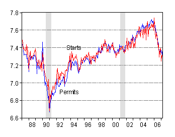
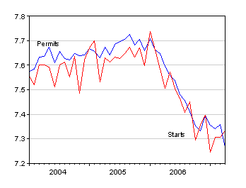
Plotted in Figure 1 is the log permits (p) and log private housing (h) starts since 1987m01. Figure 2 is a detail for the period 2004m01 to 2007m04.

Figure 1: Log housing permits (blue) and private housing starts (red), 1987M01-2007M04. Source: St. Louis Fed FREDII, accessed May 16, 2007.

Figure 2: Log housing permits (blue) and private housing starts (red), 2004M01-2007M04. Source: St. Louis Fed FREDII, accessed May 16, 2007.
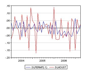
It’s certainly difficult to discern a lead-lag pattern, so in Figure 3, I’ve graphed the first log difference of each series, with permits lagged one month.

Figure 3: First differenced log housing permits, lagged one month (blue) and private housing starts, 1987M01-2007M04. Source: St. Louis Fed FREDII, accessed May 16, 2007, and author’s calculations.
Here too, it’s hard to see any clear pattern. Consequently, I’ve
resorted to statistical tests — in particular, I will rely upon a formal test for temporal precedence called Granger Causality. This is essentially an F-test for the null hypothesis that a particular variable (the first difference of lags of log permits) do not have any statistical explanatory power for current first difference log housing starts. I have conducted the test for 3 lags, 6 lags and 12 lags of first differenced log permits. In all cases, the null hypothesis is resoundingly rejected (at p-values of 7 x 10 -7, 4 x 10 -12, and 6 x 10 -12, respectively).
Now there is a difference between no and some statistical explanatory power. I undertook a more formal statistical test, which presumes cointegration between log permits and log housing starts. Specifically, I estimated this error correction model,
dht = a0 + a1dht-1+…+a3dht-3 + b1dpt-1+…+b3dpt-3 + c(ht-1-pt-1) + ut
over the 1987m01-2007m04 period, where dh is the first difference of log housing starts and dp is the first difference of log housing permits. The estimation procedure using OLS and Newey-West robust standard errors yields negative and statistically significant coefficient estimates on the ai, statistically positive coefficients on the bi, as well as a -0.16 coefficient (statistically significant at the 5% MSL) on the error correction term, viz. (h-p). The adjusted R2 = 0.31, SER = 0.055, N=244. Q-statistic tests for 6 and 12 lags failed to reject the null of no serial correlation.
The finding of a statistically negative coefficient on the error correction term is consistent with a long run relationship between housing starts and permits (in log levels). It is also consistent with housing starts reacting — in a statistical sense — to gaps between housing starts and permits. Housing permits do not exhibit an analogous relationship with the lagged gap between starts and permits.
These results lead me to the conclusion that — while permits might not be incredibly informative on their own for future housing starts — they are useful when taken in conjunction with the gap between log levels of housing starts and permits, as well as lags of first differenced log housing starts and permits.
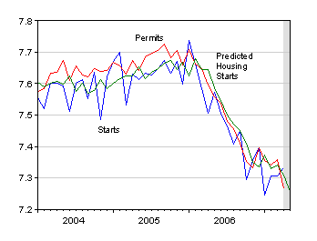
Based upon the estimated model, the predicted value for housing starts is depicted in Figure 4.

Figure 4: Log private housing starts (blue) and log housing permits (red) and predicted log private housing starts (green), 2004M01-2007M04. Source: St. Louis Fed FREDII, accessed May 16, 2007.
The model predicts continued decline in housing starts of 5.1% (in log terms), calculated as changes in predicted values (as opposed to using the actually observed value for 2007M04). Of course, with a standard error of regression (SER) of 0.055, a zero change lies within the 67% prediction interval.
More coverage on the housing release is at Calculated Risk.
Technorati Tags: housing starts, housing permits,
residential investment,
Granger causality, error correction model,
cointegration.
JDH,
The real issue is not whether permits lead starts, but whether the current level of permits/starts leads to further inventory build. I know economists are focused on the residential RE investment contribution to GDP, but there seems to be altogether too much emphasis on calling the contribution in the current quarter.
The homebuilders know full well that monetizing their land holdings in the form of spec starts may lead to further price pressures down the road. However, they have no choice if they are to service their debts, and they are also caught in a prisoner’s dilemna game whereby the one that delays starts for later may face lower margins, so they all pressure margins now by keeping starts high as an industry.
Starts that lead to inventories extend the cycle out further. That means we can expect real estate to continue to subtract from gdp until starts reach a level consistent with inventory declines. When will that be? How much of a contribution to GDP will RE invesment make in the meantime? Hard questions to answer, but the right questions to ask, IMO.
Thanks for the deeper dive Menzie. I suppose I stand corrected.
Aren’t you really just reaching the conclusion that inventories may be the best leading indicator.
Try running the same test just using inventories
to see what results you get.
When you look at the relative performance of the home builders stocks inventories are the single best variable to watch.
I’m not trying to knock your work. It looks like you may have made a significant improvement on finding a leading indicator. I’m just asking you to test another hypothesis.
David Pearson: First, clarification. I want to absolve JDH of any blame associated with this post. These are solely my own (Menzie Chinn’s) regression results. Second, I agree that stock adjustment is an important aspect of the housing market. I tried to take a first stab at that perspective in post, entitled “How big is the housing overhang”. Additional comments/critiques welcome.
GWG: I don’t think my results invalidate your view. As I tried to stress at the end of the post, the SER is 0.055, and so the information imbedded in permits still might not be very useful to the practitioner, even if according to statistical criteria, permits do have informational content above and beyond lagged housing starts.
spencer: Good point. I will try to examine this hypothesis, and get back to you. I agree there are many intersting hypotheses out there, and it’s an open question whether permits have additional explanatory power after inclusion of inventories.
Thanks to spencer for the 1-unit housing inventory data, I’m able to estimate an error correction model analogous to the one reported in the post, but including lagged inventory (k) and lagged first differencies of inventory (dk). This yields:
dht = a0 + a1dht-1+…+a3dht-3 + b1dpt-1+…+b3dpt-3 + f1dkt-1+…+f3dkt-3+ c1ht-1-c2pt-1-c3kt-1 + ut
over the 1987m01-2007m04 period. In contrast to the previous regression, I have unconstrained the long run coefficients, instead of imposing unitary elasticity between housing starts and permits. The estimation procedure using OLS and Newey-West robust standard errors yields negative and statistically significant coefficient estimates on the first and second fi, and statistically insignificant coefficients on the bi, as well as statistically significant coefficient on the lagged level terms. The adjusted R2 = 0.40, SER = 0.051, N=244.
I would therefore side with spencer‘s assertion that permits essentially do not provide additional information with respect to inventories. One caveat is that April’s inventory numbers are not currently available, while April’s permits are (thus one can’t use the equation to forecast May’s housing starts). Hence, in real-time analysis, one might be forced to rely on permits, at least until inventory numbers are released.
Menzie, here’s an “idealized” model of how starts may play out:
-in the short run, builders treat land as a sunk cost. Their marginal cost is the cost of the structure and the development. Builders will seek to build specs and gain share by cutting price as long as it is above s.t. marginal cost. Therefore starts will be only loosely correlated with HPA, inventories, etc. Also, their attempts to gain share ultimately would drive home prices towards this s.t. marginal cost.
-in the long run, builders face the marginal cost of undeveloped land, and they must estimate home prices after the development period — about four years. In a declining HPA environment and with no economic rent, there is too much uncertainty to buy land and starts collapse.
The prediction of this model is a step-function decline in housing starts. Of course it is “idealized” in the sense that builders sometimes delay building on land in the hope of better prices in the future. Perhaps this is what accounted for the initial decline in starts that we saw in 2006. Once the expectation of declining HPA sets in, however, on would counter-intuitively expect starts to stabilize (share gain) before collapsing.
The significants of inventories means that starts — or building — has to fall below sales to eliminate the excess inventories before you would expect starts to rebound.
Going forward you are going to have Web 2.0 effects. Until a year ago I worked for a building department for a large jurisdiction with a lot of new construction (no slump in the Pacific Northwest yet visible). Over the last three years they have been moving hard to move permitting on line and to eliminate redundant site visits. Given a pre-approved building plan and building in a newer approved subdivision our builders are rapidly moving to on-demand permitting, applying for and pulling the permit in the same day and actually after the start (builders often do their dirt work prior to paying for their permit and calling for their first inspections.)
The costs savings to builders in both time and money will drive this model quickly. Expect the lag between permits and starts to start to vanish. With online permitting the bigger the builder the bigger the savings. Because they can and do apply for dozens of buildings with a single online transaction and do just it time permitting. The Master Builders are probably the most politically influential group in Western Washington, they love the system and in return show their love in campaign contributions, so you can expect this trend to accelerate.
But what it does is increasingly decrease permits as a leading indicator. As permits and starts converge in time due to technological change the end result is loss of an indicator.
Nice work, Professor, and nice move to acknowledge/test/affirm spencer’s hypothesis. You’re quick, sir!
David Pearson, here is a slideshow from Lewis Alexander, the chief economist at Citigroup, which shows that the ratio of average house prices to construction cost was below 1 from 1950 to 1980. See the chart on the right side of page 4 of:
http://www.national-economists.org/news/alexander0612.pdf
Can someone please explain to me what this means, e.g. was there a home price slump from 1950 to 1980 because of high inflation? Thanks.
Thanks for investigating the statistical relationship between permits and starts. If one was to be critical the fundamental problem is that you haven’t stated a specific behavioural hypothesis. Ie why would we expect permits to lead starts? Presumably because volume and other builders have to get a permit before they can start the house. I don’t know, but that has always been my assumption.
Secondly, for my purposes, the real advantage of permits is that the Census Bureau releases them on a State by State basis each month. To the best of my knowledge you can’t easily get starts by State on line. If you could get the starts online presumably you could pick a few of the larger states, TX, FL and CA are the three largest and repeat the test at that level. If you had nothing else to do.
When I look at a Henderson (centred, weighted moving average of the seasonally adjusted data) trend of both starts and permits in year on year terms the graph suggests that USA housing has passed its worst.
Nope, only half way down. The Henderson “trend” doesn’t exist.
Charlie,
Not sure how the price can stay under construction cost for three decades. One explanation in the short run is that previously acquired land (at lower costs) is built out even while the price does not support new land acquisitions. This is a short-run phenomenon, though, as described in my post above. Over a three decade period, one would expect a price below marginal cost to coincide with minimal start activity, and this is obviously not what we observed, especially in the 1950’s.
My sense is there is something quirky going on with the NBER data he cites.
David, you are correct about something quirky with the NBER data. I looked up the original NBER paper by Glaeser et al and the answers to my question are given in note 5 on page 4 of:
http://papers.ssrn.com/sol3/papers.cfm?abstract_id=658324
I saw Lewis Alexander give his talk on CSPAN and he should have explained some of his slides better.
I am new here and first time poster. I can’t take credit for this because I read it in an article somewhere. But the housing slowdown is not near of a drag on the economy as some are predicting because of globalization. Companies that historically relied on US residential construction in this era’s economy can export much easier and economically. US exports have risen quite a bit over the past few years (would have to do research to get exact numbers) but companies such as Owens Corning (OC) are doing much more business overseas.
You might want to separate multifamily from single-family. They tend to behave differently.
The Census publishes annual data on the length of time from permit authorization to start. The 2006 data are available here:
http://www.census.gov/const/pct_auth_to_start_2006.pdf
As you can see, almost 1/2 of single-family starts occur in the same month that the permit is issued. This limits somewhat the ability of the monthly permits data to predict starts in subsequent months.
Professor Chinn, would it make sense to try to model what David Pearson says above using q-theory? (For those who don’t know, q-theory basically says that the rate of investment should be related to the ratio of the marginal value of capital to the marginal replacement cost). I found two papers which model intended housing starts via q-theory:
http://papers.ssrn.com/sol3/papers.cfm?abstract_id=911328
http://papers.ssrn.com/sol3/papers.cfm?abstract_id=410300
(Note that the first paper applies their model to the case of New Zealand where building permits happen to be called “housing consents”. Also, I don’t have access to the second paper unless I were to travel to a university library.)
David Pearson, Bruce Webb, and fnzi: Thanks for the comments. Regarding David Pearson’s alternative model, I can’t really say much. It makes sense, but the step function requires observation of data I don’t have (including expectations). I’d welcome seeing an empirical analysis of the hypothesis, or positing an econometrically testable hypothesis based on the model.
Regarding the time between permit application and house start, even if the time period shrinks, to the extent that permits are a weather-invariant variable, it might still predict subsequent starts. This temporal precedence is what I was searching for, in a somewhat atheoretical context. The fact that permits do not respond to the gap between permits and starts is supportive of a predictive aspect to permits. By the way, I fully admit that this approach was atheoretical, but there is always a tension between theory and empirics; here I took something that presupposed a link between two candidate variables, without using a fully specified model to lay out all the relationships. Doing so would have required a structural model; that in turn requires imposing many identifying assumptions, which might — or might not — be valid. And might or might not be estimable on a timely basis, given the data collected (e.q., q-theory models).
Arnold Kling: Point well taken. I’ll leave that for the next iteration; I’ll need disaggregation of permits to conform to starts for 1-unit houses.
Charlie Stromeyer: Seems like a reasonable hypothesis. The second paper looks plausible, although it’s not entirely capturing the effects laid out by David Pearson, in so far as average, measured q differs from marginal q, which is the important variable.
bmili: For certain, the demand for products that go into new houses — especially appliances — is becoming more international. But to the extent that many components of house construction are heavy (massive) relative to the cost of shipping, one still expects significant “home bias” in the production of new houses. By the way, on the “export surge”, it’s there, but slowing. See my post here as well as Brad Setser’s recent post.
Professor Chinn, if we assume competitive output and capital markets, and linear homogenous production and adjustment cost functions then marginal q = average q (or we could say that they are equivalent if producers are price takers and produce with constant returns to scale).
This is shown to be true by F. Hayashi in “Tobin’s Marginal Q and Average Q: a Neoclassical Interpretation” in Econometrica, vol 50, pp 213-24. (1982)
Is this a reasonable framework for the housing market? (I am asking because it should be easier to get average q than marginal q).
Charlie Stromeyer: Absolutely, those are the conditions that will make average and marginal q the same. I think there is a deeper question, related to the “Two Cambridges” issue, which as I recall is whether capital can be aggregated. Assuming for the moment it can, then there remain measurement issues as well (see Desai-Goolsbee article cited in an earlier post). I might also note that the pure investment function associated with neoclassical q-theory cannot be estimated since adjustment is instantaneous. Only by assuming adjustment costs (quadratic in the Summers 1981 BPEA paper) can one estimate the investment function.
I must admit I don’t have a good idea whether the assumptions are appropriate for housing or not.
Professor Chinn, the “Two Cambridges” capital controversies were not originally solved but were instead swept aside as neoclassical economics became orthodoxy. However, Felipe and Fisher revisit this issue and discover that aggregate production functions don’t work:
http://papers.ssrn.com/sol3/papers.cfm?abstract_id=422067
As for measuring q, I will take a look at the Desai and Goolsbee article. I like the paper “On the Accuracy of Different Measures of q” by Erickson and Whited which is available here:
http://papers.ssrn.com/sol3/papers.cfm?abstract_id=938718
For anyone who might be interested here is a free copy of the Felipe and Fisher paper above:
http://are.berkeley.edu/courses/ARE241/fall2005/Felipe.pdf
Here is a more recent paper by Temple which argues that the critique of aggregation is more serious for empirical research than for theoretical modeling:
http://www.econ.iastate.edu/tesfatsi/AggregProdFunctionsDontExist.Temple.pdf
Also, here is a new paper which adapts Hayashi’s model to include financial frictions:
http://econ-www.mit.edu/faculty/download_pdf.php?id=1026
Finally, this is something I don’t know:
Is the relative change in the number of housing starts higher(lower) during a boom(bust) than during a normal market?