Time for an update on estimated income and price elasticities of US trade flows. These issues are important to those of us who believe that the US remains vulnerable to shifts in the rest-of-the-world’s willingness to finance the current account deficit. If you think it’s just jolly fine and likely for the US to keep on borrowing at around 6.5 percent of GDP for the indefinite future, skip this post.
In my previous post on the subject, I focused on implications of the income elasticity estimates for secular trends in the trade balance/exchange rate relation. In this post, I report results from a newly revised paper [pdf], focusing on the price elasticity estimates, much like the recent IMF’s World Economic Outlook Chapter 3 [pdf] did.
First, to place matters in perspective. Figure 1 shows the US trade balance to GDP ratio (red) and the ratio ex-oil (green), against the log broad trade-weighted real dollar exchange rate from the Fed, lagged two years.
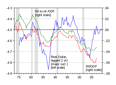
Figure 1: Log real broad trade-weighted dollar (blue), trade balance to GDP ratio (red), and ex-oil trade balance to GDP ratio (green). NBER-defined recessions shaded gray. Source: Federal Reserve Board, BEA (April 27 release), and NBER.
The graph highlights the difference between this and the previous adjustment episode. In the previous episode, the trade balance — defined either way — responds two years after the peak of the dollar. In the most recent episode the total trade balance responded about 4 years after the dollar peak in 2002, while the non-oil balance responded some 2.5-3 years after the peak.
Many factors — even in the limited partial equilibrium framework I’m going to use — can cause this divergence. One factor is diverging income trends in the US and the rest-of-the-world (RoW) as well as differential income elasticities.
Using a very standard trade equation framework, I estimate the following relationships for exports and imports.
ext = a0 + a1ytRoW
+ a2qt
imt = b0 + b1yt
+ b2qt
Where a1 > 0, a2 > 0, b1 > 0, b2 < 0. y is an income variable, and q is the real exchange rate.
The results obtained from estimating these equations using dynamic OLS (no trend) are depicted in Figure 2 for income elasticities. The dashed lines are the full sample elasticities, while the bars denote the estimated elasticities for the indicated subsamples.
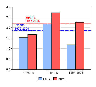
Figure 2: Export income elasticity (blue) and import income elasticity (red); dashed line is DOLS estimate for entire sample, bars are for indicated subsamples. Source: author’s calculations.
Notice in Figure 2, the import elasticity exceeds the export. This is merely a reconfirmation of the existence of the Houthakker-Magee result. The existence of this asymmetry means that even if income growth is relatively the same at home and the RoW (Figure 3 depicts the log real GDP levels in the US and abroad), the trade deficit will widen even with a constant real dollar exchange rate.
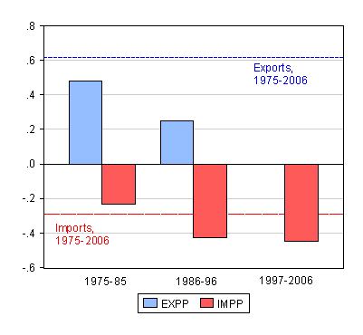
Figure 3: Export price elasticity (blue) and import price elasticity (red); dashed line is DOLS estimate for entire sample, bars are for indicated subsamples. Source: author’s calculations. Note: price elasticity refers to response to real exchange rate.
Notice that if one breaks the overall sample into roughly three equal subperiods, the income elasticity asymmetry does not seem to be disappearing. If anything, the gap seems to have widened in the 1997-2006 period.
Price (actually exchange rate) elasticities are shown in the next figure. The full sample estimated export elasticity is substantially larger than the (absolute value of the) import elasticity. In other words, it appears more difficult to reduce imports than expand exports via expenditure switching.
The subsample estimates are quite hard to interpret. Except for the first subperiod, they do not match the stylized fact I have just mentioned. I will argue that this is likely to be an artifact of inappropriate aggregation of the data.
For instance, for US exports, one could look at total exports of goods and services. Or one could look at goods and services separately. And even goods, it could be argued, are sufficiently heterogenous that one might want to pull out agricultural goods. Or capital goods. Or both agricultural and capital goods. For imports, one might want to do the same (except pull out oil instead of agricultural goods). I show these goods subcategories in Figures 4 and 6.
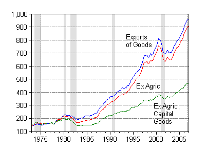
Figure 4: Real exports of goods (blue), ex-agricultural goods exports (red), ex-agricultural and capital goods exports, in billions of Ch.2000$, SAAR. Source: BEA (April 27 release).
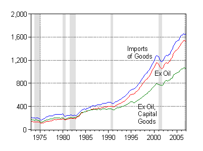
Figure 5: Real imports of goods (blue), ex-petroleum goods imports (red), ex-petroleum and capital goods imports, in billions of Ch.2000$, SAAR. Source: BEA (April 27 release).
Now, one can easily observe that imports and exports excluding capital goods exhibit substantially different behavior than total trade flows, particularly around the 1999-2001 period. Alternatively, capital goods imports and exports appear to be correlated with equipment investment in those years.
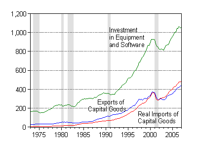
Figure 6: Real exports of capital goods (blue), real imports of capital goods (red), and real investment in equipment and software, in billions of Ch.2000$, SAAR. Source: BEA (April 27 release).
Theory, as discussed in my previous post, suggests that as trade and transportation costs decline, vertical specialization which involves importing goods to produce goods for export, will increase. Indeed, work by Kei-Mu Yi pdf] suggests a nonlinear relationship between tariffs rates and vertical specialization. In the subsequent figure, I show the nominal shares of goods trade associated with capital goods, against the G-3 average tariff rate.
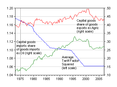
Figure 7: Tariff factor squared, viz., (1+t)2 (blue), capital goods share of non-agricultural goods exports (red), capital goods share of non-oil goods imports (green), SAAR. Source: Kei-Mu Yi, and BEA (April 27 release).
There does seem to be some link, inspiring formal estimation of trade flows accounting for these effects. In the paper, I find that ex-oil import prediction errors are substantially smaller when one estimates the comonents, then sums up the components into aggregates. Over the 1990-2007q1 period, the mean error is $21.61 billion versus $41.14 billion; in percent terms, RMSEs are 4.1% versus 6.1%.
In this post, I wanted to focus in on the question of what happens to the implied price elasticity when one disaggregates, and incorporates a role for vertical specialization in the specifications. I do this by adding equipment investment and a tariff factor into my equations. In contrast, the authors of Chapter 3 of the WEO incorporate sector-specific exports into the sector import equation at a more disaggregated level.
I find that a 10% dollar depreciation yields approximately a 1 percentage point of GDP improvement in the real trade balance, when using the conventionally estimated equations. A 1.7 percentage point improvement occurs when taking into account the fact that capital and noncapital goods imports differ in their behavior. (A subtlety is that the exercise is conducted assuming that income and capital investment remain unchanged as the exchange rate changes, so this is a ceteris paribus.)
Interestingly, while my estimate of the required depreciation under the alternative specification matches the IMF’s, my estimate for the baseline specification is only about a third of the IMF’s corresponding estimate. Hence, my modifications do not imply such a substantial alteration in the implied required amount of exchange rate depreciation, but they still do imply some room for greater optimism, should incipient capital inflows decline.
Technorati Tags: dollar,
exchange rate,
trade deficit,
capital goods,
vertical specialization.
10% for 1% was — funnily enough — Ted Truman’s rule of thumb back when i was at the treasury. it was usually expressed as 10% for $100b, or $1% = $10b, but if you adjust for changes in the size of the economy, it works out to the same thing.
Nice work, Professor Chinn. You might also be interested to know that the price (exchange rate) elasticities approach will not work for countries such as China. McKinnon and Schnabl explain why on page 9 of their paper:
http://papers.ssrn.com/sol3/papers.cfm?abstract_id=905503
Brad Setser: Yes, it is interesting how durable these rules of thumb are. When I at CEA, that rule also floated around. But I think that rule conflated both price and income effects that were typically associated or correlated with large exchange rate depreciations.
Charlie Stromeyer: I know both McKinnon and Schnabl and respect their work. And there are definitely elements of truth in there arguments, as the channels they discuss are now laid out in the standard international textbooks (see Caves, Frankel and Jones, e.g.,), but in reverse (usually for discrete devaluations). But most calls now are for a more rapid rate of CNY appreciation, not for large discrete revaluations. Moreover, most of the overseas assets owned by China are held by the Chinese government — not clear to me how they internalize that wealth.
There are measurable effects of exchange rate changes on Chinese exports. Whether there are for imports remain to be seen. See these posts, and the papers cited therein: [1] and [2].
Professor Chinn, it is not clear to me either how the Chinese government would internalize that wealth but I have heard two reasons why they accumulate such large forex reserves:
1) China is the world’s third largest importer. BusinessWeek says that having a huge stash of hard foreign currency is needed in the event of a major crisis, i.e. it is a huge rainy day fund. This is because the Chinese could use the foreign currency to buy the imported materials and equipment needed to keep their factories going (without having to resort to borrowing money).
2) Richard Cooper of Harvard University says that investing domestic savings in US dollars makes good sense for a country such as China because they have insecurity of property rights.
Charlie Stromeyer: With respect to (1), the “self-protection” explanation made sense during part of the period of reserve accumulation. However, the over $1 trillion in reserves seems far in excess of what’s needed in case of a “sudden stop” (which is not much of a worry for a country with a $200 billion or so current account surplus).
Point (2) is a common element to the Bernanke saving glut thesis, as well as arguments posited by Rich Clarida and Glenn Hubbard, among others. For my views on this approach, see this post.
Professor Chinn,
I don’t know if you noticed, but your paper on the Yaun got mentioned in the Economist a couple of weeks ago.
Congratulations.
Prague Twin: Yes, I had seen that (although quite brief, so one could have easily missed it). Thanks for the note.