As the U.S. economy goes into a downturn, we are going to be reminded that extrapolating trends is a hazardous enterprise. For instance, linear extrapolation of tax receipts (expressed as a share of GDP) is probably something that one should be wary of doing. And yet, as shown in some comments on previous posts (see here and here), there seems to be too much belief in what ocular regressions can tell one.
So here is post that, while it seems to be completely unrelated to issues of current interest, should be of concern to those who do forecasting. (Time series econometricians can skip this post, or you will be appalled at the things I’m going to say, in terms of the sloppiness of discourse. The technically inclined should read Jim Hamilton’s book, chapters 15-17.)
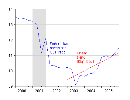
Let me return to the issue of Federal tax receipts (line 2, BEA GDP table 3.1) expressed as a share of GDP. Back in July 2006, I asserted that the increase in tax receipts was not so remarkable in the context of statistical uncertainty. A cursory glance at the data would seem to contradict my assertion. Indeed, the sky seemed to be the limit in July 2006.

Figure 1: Federal tax receipts to GDP ratio (blue), and linear trend estimated over 2003q1-06q1 period (red). Source: BEA NIPA release of 29 November 2007, Table 3.2, NBER and author’s calculations.
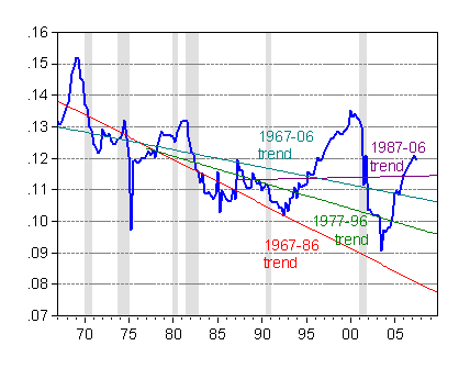
What troubled me was that the discourse was couched in terms of trends and period averages. I mentioned that estimated trends were sensitive to sample period. And here is an illustration of that fact. I’ve plotted below estimated (OLS) linear trends for several different superiods. One clear result is that the “trends” move around with the sample period.

Figure 2: Federal tax receipts to GDP ratio (blue), and linear trend estimated over 67q1-86q4 period (red), 77q1-96q4 (green), 87q1-06q4 (purple) and 67q1-06q4 (teal). Source: BEA NIPA release of 29 November 2007, Table 3.2, NBER and author’s calculations.
The sensitivity of estimated trends to sample periods is the quintessential feature of nonstationary time series, or more precisely integrated time series (a random walk is an example of an integrated time series). Technically, the OLS estimator of the trend coefficient does not converge to the population mean when dealing with an integrated series.
Now one might argue that the tax receipt to GDP ratio cannot literally be a nonstationary series; it’s bounded from below at zero and above at one. However, the question is whether over the sample period is bounded; or even if the series is stationary, but highly persistent, then one might still get this outcome.
What do formal tests indicate? A standard unit root test (ADF, using the Schwartz Bayesian information criterion for lag length, and allowing for constant and trend) fails to reject the null hypothesis. Using the Elliott-Rothenberg-Stock Dickey-Fuller test also fails to reject the unit root null. The Kwiatkowski-Phillips-Schmidt-Shin (KPSS) test which has a trend stationary null rejects at the 5% MSL (bandwidth for the kernel estimator is 10). In other words, the series is so persistent that it is better treated as an integrated process than as a trend stationary process (no surprise to people who work in the macroeconometrics). On the other hand the change (i.e., first difference) of the tax receipts/GDP ratio is stationary (or technically, rejects the unit root null, and fails to reject the trend stationary null). Hence, the Federal tax receipts to GDP ratio appears to be difference stationary.
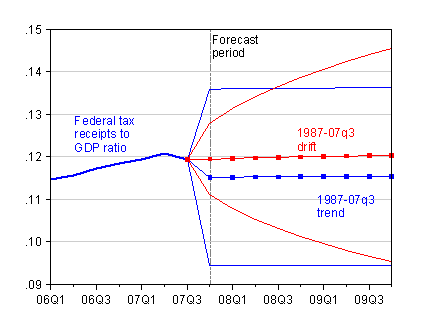
So, reader, beware of fitting trends and extrapolating! What’s the recourse? When the series is difference stationary, then one can forecast by working with the first differenced series. I show the implications of doing so in figure 3. The blue line with boxes is the forecast using a linear trend; the red line with boxes is the forecast assuming the ratio “drifts” up over time (technically, here I’m modeling the ratio as a random walk with drift, although a more refined approach would probably model the series as a ARIMA(0,1,1)).

Figure 3: Federal tax receipts to GDP ratio (blue), and linear trend estimated over 87q1-07q3 period (blue) and plus/minus 2 standard error prediction intervals; and forecast from estimated drift (red) and plus/minus 2 standard error prediction intervals. Source: BEA NIPA release of 29 November 2007, Table 3.2, and author’s calculations.
I’ve included the ±2 standard error bands for the respective forecasts. One interesting aspect is that the prediction interval expands over time for the difference stationary forecast (in red). The prediction interval for forecast assuming trend stationarity does not expand over time. Of course, the test results suggest that the assumption of trend stationarity is not justified, so the prediction interval is included merely for illustrative purposes.
The key take-away from this last figure is that even when the forecast trends are very similar, the implied uncertainty regarding the forecasts values differs substantially. In the figure, the two forecasts just happen to parallel. However, the more appropriate forecast associated with the difference stationary assumption implies much greater uncertainty going out toward longer horizons. Assuming trend stationarity (when not appropriate) provides an false sense of certainty.
For more (albeit dated) cautionary tales, see “Beware of Econometricians Bearing Estimates,” JPAM (1991).
Technorati Tags: tax revenues,
trends,
stationarity,
random walk,
unit roots,
forecasts.
I mentioned that estimated trends were sensitive to sample period.
That’s exactly what I found when I did the regressions on the GDP ratio in the other post. Just starting the regression in Q1’04 vs. Q2’03 made a huge difference in the slope. Big change in R^2, too.
I think that you can see the increase in spending due to the Iraq war in the data, starting at the end of ’03. The increase in spending is competing with the increase in GDP for control of the ratio. Maybe you see a little more randomness in the graph than in previous time periods as a result.
Bravo for putting uncertainty measures around your forecasts! (You’re probably also the only blogger I know of that will tell time-series econometricians to skip the post, then mention the bandwidth parameter on the KPSS test :-))
I’ll note an important implication of the issue that you raise; because estimates of recent trends are uncertain, so are estimates of recent cycles. This is critical for macro policy, where so much emphasis is put on correcting deviations from “equilibrium” levels. (Think of exchange rate over/under valuation, estimates of “structural” fiscal deficits, or just estimates of the business cycle.) Orphanides and van Norden (REStat 2002 or an earlier working paper version at http://ideas.repec.org/p/fip/fedgfe/1999-38.html) show the seriousness of the problem for various methods of estimating output gaps. Mishkin (2007 at http://www.federalreserve.gov/newsevents/speech/mishkin20070524a.htm) gives an excellent discussion of the problem for monetary policy. For the more technically minded, van Norden (2002 at http://ideas.repec.org/p/bca/bocawp/02-28.html) formalizes the problem in the frequency domain and shows how the seriousness varies across the common problems of estimating recent core inflation, trend productivity growth and output gaps.
I’ll also note one other fly in the ointment; data revision. If we acknowledge that GDP and tax revenue estimates tend to get revised and that the most recent estimates are the least reliable, then forecasting becomes trickier still and the uncertainty increases. For some series (e.g. CPI, unemployment, stock prices, exchange rates) this problem is non-existant or trivial. For other series (e.g. Balance of Payments, investment, productivity, government finances) the problem is much more serious.
A trend is a trend is a trend,
The question is, will it bend?
Or change its course,
Through some unforeseen force,
Or carry along to its end.
Just in case readers wonder why receipts are such a small share of GDP, I would just note that the “tax receipts” you are plotting exclude social security contributions. The NIPA-defined taxes are personal and corporate income taxes plus excise taxes, custom duties, and Federal Reserve earnings.
Buzzcut: Yes, although in the case of Federal current expenditures, the nonstationarity is more obvious. Here, I’m looking at NIPA defined tax revenues, which look more trend stationary, and trying to show that even here, one has to be very careful.
Simon van Norden: Thanks for the compliment and for the references. I think you bring up an important point. Only one type of uncertainty is highlighted here — what is the right specification, and hence the right prediction intervals to place around the forecasts? However, as you point out, there is the additional problem of how to account for data revisions. For US data (presumably others as well), there are three releases for NIPA related data, and then comprehensive revisions that extend years back. As I’ve pointed out in previous posts, these revisions can change the time profile for various series, especially around turning points (see here). The problem is even more complex when one considers regressions with right hand side variables (besides trends), since then one has both measurement error and revisions on both sides of the regressions.
rana: Good point. Thanks for the clarification.
I’ll only think we are headed into a recession when the ECRI, with Laxman Achutan and Anirvan Banerji, say we are entering a genuine recession.
Menzie,
Good bridge between econometrics and economics for the man-on-the-street. Well done. A couple of points, since you are using quarterly data a more appropriate model might have been ARIMA (0,1,1 0,1,1)….or perhaps not if the data were already seasonally adjusted. Also, I seem to recall reading a paper you wrote awhile ago that relooked the Nelson-Plosser controversy using quarterly versus annual data. If I recall correctly you found that using quarterly GDP data was more likely to show unit roots (stochastic shocks had a lasting effect) than annual data, which showed a more deterministic trend. Of course, that was GDP data and not tax receipts as a percent of GDP, but I wonder how much of the nonstationarity is due to quarterly data versus annual data.
GK: The post eschewed the word “recession”. Don’t forget Jim Hamilton’s recession indicator.
2slugbaits: I am impressed that you would remember the results from a decade-old paper (JBES, 1997). The reason why Yin-Wong Cheung and I were able to distinguish between trend vs. difference stationarity in the annual, but not quarterly, data was we believed due to the longer span of data (over 100 years) available at the annual frequency. We provide additional cautionary tales regarding local currency versus PPP GDP measures (such as in the Penn World Tables) in our 1996 Oxford Economic Papers article.
Income tax receipts have been buoyed by the rapid increase in corporate income as a share of National Income and the increasing share of wages at the top of the income distribution. Unless one expects these trends to continue the growth in receipts as a share of income will not continue.
As an ex-pro market technician, it reminds me of the old joke
“What does a technician do when prices break the trend-line?”
(draw a new trend-line)