This is the second of two posts (first can be found here) based on the Craig Hiemstra Memorial Lecture that I’ll be giving in San Francisco on Friday. There I’ll be discussing some ongoing research I’ve been doing with Mike Owyang of the Federal Reserve Bank of St. Louis on regional propagation of business cycles.
I earlier described some of the patterns found when you apply the algorithm used to construct my GDP-based recession probability index to individual state employment growth data. Last week’s colorful moving gifs were calculated by applying that algorithm to each state individually in isolation from all the others.
One could in principle apply exactly the same method to the full vector of states at once, as could be described if you’ll indulge in a little notation. Let yit denote the employment growth rate for state i in quarter t. I’ll use N for the number of states– our empirical analysis only uses the N = 48 contiguous states. Let yt = (y1t,y2t,…,yNt) denote the full (N x 1) vector of observed employment growth rates for all the states for quarter t. Let sit = 1 if state i is in recession in quarter t and sit = 0 otherwise and st = (s1t,s2t,…,sNt). We don’t observe sit directly, but it influences the observed data yit in a particular hypothesized way, allowing us in principle to characterize the conditional density
f(yt|st) and use Bayes’ Law (just as in the scalar case) to calculate the probability that st takes on any particular value conditional on observing all the data for all the states at all dates. The problem is that there are 2N = 281,474,976,710,656 different possible values that st can take on, making such inference completely infeasible in practice, even though with vector notation it seems easy enough to write down the equations you’d want to use (specifically, equations [22.4.5] and [22.4.6] in my text where P has 2.8 x 10¹⁴ rows and columns, if you’re asking).
The approach that Mike Owyang and I have taken is based on the premise that most of these 2N possibilities will never happen. Instead, we assume as in Fruhwirth-Schnatter and Kaufmann (2008) that states tend to move together in clusters, so that there is a small number K of possible values that st might assume. We’ve had the best success so far with K = 5. We take two of these possible configurations (which we label by 4 and 5 respectively) to be the natural ones, where in (4) every single state is in expansion at the same time and in (5) every single state is in recession at the same time.
For the other 3 configurations, we let the data tell us which group (if any) state i is most strongly associated with, viewing the cluster affiliation of state i as another unobserved random variable about which we’ll draw an inference based on the observed behavior of state employment growth rates. Details of exactly how we do that would probably not be of interest to most Econbrowser readers, but hopefully for my Friday audience– the 16th Annual Symposium of the Society for Nonlinear Dynamics and Econometrics— it will be right up their alley.
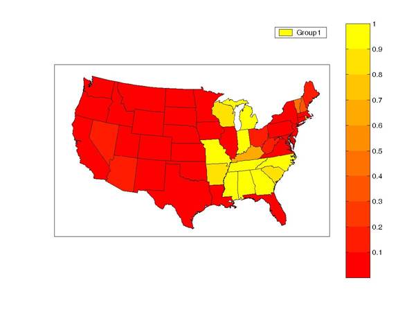
Here’s a quick look at some of the results we obtained. Cluster 1 states sometimes tend to go into recession one quarter before the rest of the country. These states are concentrated in the southeast and midwest. The color on the graph below displays the Bayesian probability, based on the observed employment data, that an individual state is part of cluster 1, with brighter yellow indicating a stronger association with this group.
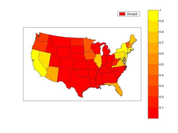
Employment growth for states in the second cluster sometimes recovers more slowly after a recession than for other states. Cluster 2 states (indicated by yellow on the graph below) can remain in recession for several quarters or even years after most other states have begun their recovery. California and several states in the northeast appear to exhibit this pattern.
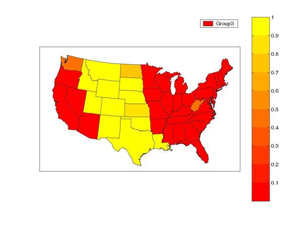
The third group can go into recession even when the rest of the economy avoids a downturn altogether. This cluster consists of the mountain and plains states. A big part of their separateness seems to be their regional recession during the collapse in oil prices in the mid 1980s.
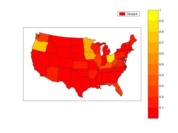
The fourth group consists of states that only are in recession when every other state in the country is in recession. A bit surprisingly, our estimates suggest that this “just-like-everybody-else” status is in fact quite unusual.
We then used all the states together to calculate the probability of any one of the K possible outcomes at every historical date. The blue line in the figure below shows the probability that states characterized by cluster 5 (in which every state is included by definition) experienced a recession at that date. This is quite similar to the NBER national recession dates, although the 2001 downturn is judged much longer when you look at employment growth rather than GDP growth (the “jobless recovery” on which many have commented). It’s also interesting that state-level employment data would lead you to conclude that another national recession began in 2007:Q2. I don’t want to put too much emphasis on that last result, since we have made no effort to capture changing employment dynamics over time or take account of the difference between revised and real-time data. Moreover, these results are still quite preliminary. Nevertheless, the latest spike up in the recession probability does not look like an irresponsible assessment at the moment.
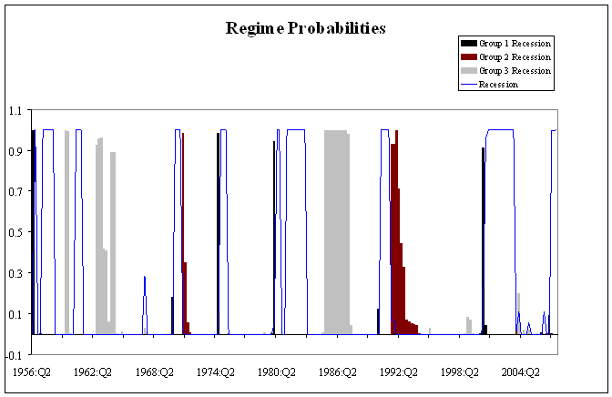
The above graph also underscores a comment I made last week— recessions can be quite different from each other. For example, only the 1974, 1980, and 2001 recessions clearly began with the cluster 1 states, while the slow recovery of the cluster 2 states primarily reflects the patterns in the 1970 and 1991 recessions.
It’s interesting that a phenomenon as recurrent as the business cycle can have such a different look each time it comes around. The current episode should be no exception.
Fascinating, Professor!
I wonder how to characterize these groups. 1 manufacturing, 2 finance/tech, 3 commodities, 4 ?
“Cluster 2 states (indicated by yellow on the graph below) can remain in recession for several quarters or even years after most other states have begun their recovery. California and several states in the northeast appear to exhibit this pattern.”
I think it’s interesting that the States that are slowest to rebound, the case can be made, are the ones with the largest Government burden-taxes, regulation.
How about applying a Monte-Carlo type simulation and see how well that matches with your clustering approach? In my experience, this can be very useful as long as you do a reasonable number of simulations (> 100,000).
mjc, our estimation method is Monte Carlo Markov Chain. I apologize that we still don’t have a copy of the paper posted for people to follow details of the algorithm.