Over the past few days, I’ve been trying to identify appropriate measures of the output gap (and trying to relate that to exchange rate changes). As I’ve done so, I’ve come to realize that (1) it’s a difficult thing to do, and (2) interesting stories come out of different measures.
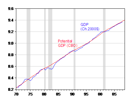
The easiest thing to do is to pull down the CBO’s measure (interpolated to quarterly frequency). This yields the following picture (in logs):

Figure 1: Log real GDP (Ch.2000$, SAAR) (blue line), and log potential GDP. NBER-defined recession dates shaded gray. Source: BEA, GDP release of 29 May 2008, and CBO, Update of CBO’s Economic Forecast (February 2008), data [xls], and NBER.
Two observations: (i) recessions do not necessarily coincide with negative output gaps (although they do seem to coincide with the beginning of periods of negative output gaps); and (ii) recoveries do not always coincide with positive output gaps.
This is obvious when one thinks about it, given the NBER BCDC definition of a recession as the following:
A recession is a significant decline in economic activity spread across the economy, lasting more than a few months, normally visible in real GDP, real income, employment, industrial production, and wholesale-retail sales. A recession begins just after the economy reaches a peak of activity and ends as the economy reaches its trough. Between trough and peak, the economy is in an expansion. Expansion is the normal state of the economy; most recessions are brief and they have been rare in recent decades.
That is a recession is the description of the first derivative of output taking on a negative value, while an output gap is a description of output relative to the output level consistent with the “normal” utilization of factors of production (also “full-employment”). For details of how CBO calculates potential GDP, see this document.
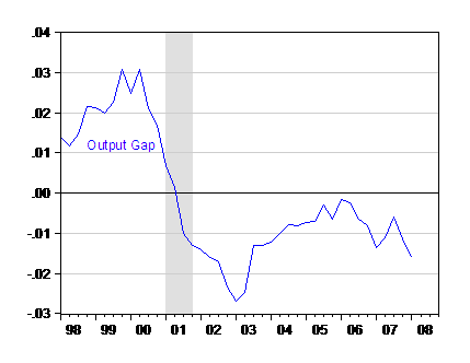
Looking at the last ten years provides another insight.

Figure 2: Log real GDP (Ch.2000$, SAAR) minus log potential GDP. NBER-defined recession dates shaded gray. Source: BEA, GDP release of 29 May 2008, CBO, Update of CBO’s Economic Forecast (February 2008) [xls], NBER, and author’s calculations.
The US economy only barely made it close to full-employment in the expansion of 2001-2007/8/?, and is now declining again. I think I had realized this (especially in the course of various past debates over the surge in tax receipts, which I think has now been resolved — see [1], [2] for a recollection.)
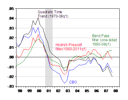
As I noted in the beginning of this post, I was finding it difficult to discern the most appropriate measure, so I will share the other measures I have investigated as indicators of potential (or “trend”) GDP (which can then be used to calculate corresponding measures of the output gap): (1) the Hodrick-Prescott filter; (2) the Band Pass filter; and the quadratic time trend.
The Hodrick-Prescott filter is a ubiquitous two-sided filter used in time series macroeconometrics and elsewhere (I’ve even seen it used in the analysis of temperature data! [3]). Essentially, the HP filter calculates a trend that minimizes the weighted sum of squared deviations from trend, and squared changes in the the growth rate of the trend. This weighting is controlled by a parameter which is usually set at 1600 for quarterly data. As a public service, I’ll note there are serious hazards associated with this filter, especially when trying to correlate various macro series that have been put through the same filter [4].
There is an additional problem (which is often ignored), namely that the HP filter is two-sided, so that running the filter up to the end point of data will tend to result in the trend being too close to the last data point (in our case, the output gap will be pulled to zero).
There are several band pass filters; the one most commonly used in the macroeconometric literature is the Baxter-King version.
Band pass filters are called this because (in the frequency domain) they pass through any cyclical components within a particular frequency band, and elimates the others. In the time domain, this means fluctuations that are shorter or longer than a specific length are ignored. In the business cycle area, then, in order to use this filter, one would have to have a prior on how long a “typical” business cycle is. More on both the HP and BP filters can be found in Tim Cogley’s entry for the New Palgrave Dictionary of Economics [5].
The final means of identifying the output gap is to the simplest (at least in implementation) — take the deviation from an estimated quadratic trend in time. This is not an uncommon procedure, but if you are pretty confident there is a unit root in log GDP, you might feel a little queasy about doing this [6]. But for completeness’ sake, I’ll show what happens when you do this as well.

Figure 3: Output gap measured as deviation from CBO potential (blue), HP filter (red), BP filter (green), and quadratic time trend. Source: BEA GDP release of 29 May 2008; Update of CBO’s Economic Forecast (February 2008), data [xls], NBER, and author’s calculations.
Note that in order to circumvent the two-sided filter aspect of the HP filter, I have done a standard fix, which is to use an ARIMA(1,1,1) on log GDP over the 1980-08q1 period to dynamically forecast out 12 quarters, and then apply the HP filter to this “extended” series. I could have done a similar procedure for the BP filter, but opted to use the Christiano and Fitzgerald (2003) one-sided asymmetric version of the band pass filter to estimate the trend series.
First, the good news. Using the band pass filter, one finds that the output gap is still positive, at less than one percentage point of GDP in 2008q1. The HP filter indicates an essentially zero output gap. The quadratic trend indicates something similar to what the CBO indicates — something close to a 2 percentage point negative output gap in 2008q1, versus 1.5 percentage points for CBO.
I don’t want to say that there is one best version. Variations in the sample period, and the parameters used in each filter, will change the results. And of course, data revisions will mean the real-time output gaps will differ from the final revised output gaps we estimate today using either mechanical or judgmental approaches. For a pessimistic view regarding real time use, see Orphanides and van Norden (2004) [pdf].
Nonetheless, the distinction between the rate of change in economic output, and where output levels will gravitate to (and at what pace) is a useful one. And I think it will become of greater usefulness as the slowdown ends, if and when growth resumes. In particular, I’m thinking of whether the pattern of smaller — but more persistent — ups and downs continues (the half life of a deviation from potential has risen from 8 quarters in the 1970-90q1 period to 11.6 quarters in the 1990q2-2008q1 period).
[Update – 3pm 12 June]
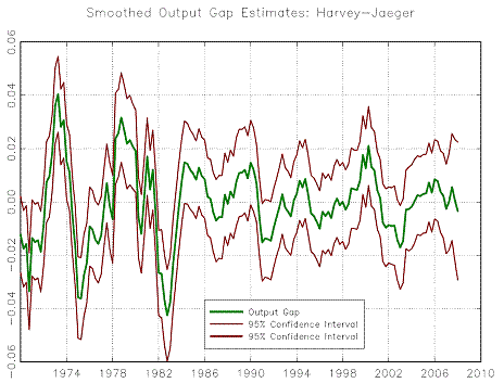
Simon van Norden (aka SvN) has taken up the challenge, and provided a graph depicting the output gap plus a 95% confidence interval. He writes:
Your recent post got me interested enough to update some of my code on estimated output gaps. I’ve attached the resulting graph in PDF and PS form; please feel free to post either one.
I downloaded the latest real GDP figures from FRED (GDPC96) and fit the log of the series using Harvey-Jaeger’s (JAE 1993) model; this allows for time-variation in the growth rate of potential plus cyclical dynamics. While other univariate state-space models can give similar results, they found that theirs gave results for the US that were very similar to those of the HP filter. The graph shows our best estimates of the cyclical component of their model (a.k.a. the output gap) as well as its 95% confidence interval. [Technical note: These are the smoothed estimates, so we see the confidence intervals flare out as we get close to the end of the sample. Also note that these include parameter uncertainty using the Ansley-Kohn method; in this case Hamilton’s method gave almost identical standard errors.]
The graph shows that variations in the estimated output gaps over the past 3-4 years are dwarfed by their confidence intervals (although, to be sure, the latest data point shows a move from above potential to below.)

Figure 4: Smoothed output gap, per Harvey-Jaeger (2003). Source: personal communication, Simon van Norden.
The underlying article can be accessed via JSTOR, here.
Thanks, Simon!
[Late update: 16 June]
Caroline Baum has a interesting artice discussing the schizophrenic nature of economic announcements in these times. See
“Market Mood Swings From ‘Om’ to OMG! and Back”.
Technorati Tags: potential GDP,
recession, output+gap,
full employment output, trend.
How Do Oil Prices Compare in Other Currencies?
Menzie Chinn submits: Some of the explanations for the dollar jump rely upon the perceived weakness in the dollar’s value (and hence, by extension, Fed policy). Does this make sense? As I’ve remarked before [1], there is likely a two way causality betwe
MC, there’s been something I’ve been looking at in my studies (that I think is important) and it’s illustrated in your first chart.
In four of the five recessions shown, GDP rose above potential *first*, *before* a recession came along.
Just a layman’s point of view, but doesn’t expansion beyond potential mean an overheated economy that will become inflationary, which will demand aggressively tighter monetary policy, which will in turn bring about recession?
(Just as an aside, I have serious doubts about the current/imminent recession argument that’s floating around for this very reason: The economy never reached that “overheated” stage, so how can the business cycle come to an end with recession?)
Sebastian
Hi Menzie,
I love your posts. I find them very interesting and I learn a lot.
Regarding the output gap, is there any software that computes the band pass filter a la Baxton-King? Or at least a matlab code or something like that? That would be very useful!
The other two are easier to implement once you take into account the caveats that you mentioned.
By the way, have you found any interesting relationship between output gaps and exchange rate changes as you mentioned in the beginning of this post?
Thanks a lot
Whenever you put a point estimate (forecast) out there you should put upper and lower confidence limits on it. Furthermore if you are trying to conclude that the output gap is actually above zero you need to do a hypothesis test that takes into account the error in your forecast. While your analysis appears to be rigorous on the surface, it is anecdotal unless you do a hypothesis test.
With that said you have some very interesting information here.
The failure of output to exceed its long-run potential is right in line with weak job creation in this cycle. It also suggests that, while we may have missed some illegal hiring in the official data, we haven’t done all that badly. Hiring and output both fell below average in the official data for this cycle.
The implication to this is that the downturn is likely to be less severe because output and employment don’t have to fall to trend before falling below trend, yes? A shallow slowdown because amplitude on the downside reflects amplitude on the upside.
Sebastian,
See the prior post – “Trends in Key Recession Indicators”. Your question about whether recession is possible when output has not run above trend is possible. Also note that the mechanism you specify, in which overheating leads to a central bank tightening, has to do with credit tightening. Credit has tightened due to disintermediation and tighter lending standards, and central banks are pretty clearly considering tighter policy despite slower growth. The mechanism you specify to generate recession is at work, and may be intensified by central bank action.
Alejandro:
Go here http://www.clevelandfed.org/Research/Models/bandpass/index.cfm
for Matlab codes.
Ed: Point well taken. Of course, for a quadratic in time trend, there are no “correct” standard errors, if the true dgp is I(1). Otherwise, they’ll be pretty tight, I’d guess. I’ll leave it to you to do the standard errors for the others (which will entail a number of additional assumptions). I look forward to seeing what you generate.
Hi Menzie,
The perfect econ blog post. Thanks.
That’s all we got for the trillions….
By Fester: The US economy is in recession for most people. Either their disposable income is getting compressed due to high price increases in hard to substitute goods such as fuel, energy, food, education and healthcare, jobs are being lost
I have my doubts about CBO’s estimation of potential, which appears visually to rise at a faster rate in the 1970s, late 1980s and late 1990s, while rising at a slower rate in the other periods. Details in their assumptions are, for example, here. They apparently average out over decades the rises and falls seen visually to show a falling potential output.
Some of the data are probably pretty good, like business investment. Others should be good, like labor force size, but with so many undocumented immigrants the uncertainty could be larger than one imagines. Others, like potential labor force productivity, probably have large uncertainties associated with errors in numerator and denominator. Also, there’s a squishiness associated with the fact that the size of the potential labor force is affected by decisions to pursue education or child rearing.
So, Menzie, how about this possibility: that the real item of interest is falling potential; further, that GDP has been falling further and further below where potential should have been since the 1970s?
Sebastian: The logic you laid out makes sense if the only shock that hits the economy is monetary policy responding to inflationary pressures arising from excess aggregate demand. But if there are supply shocks, for instance, one could imagine negative output gaps without the benefit of a preceding positive output gap. This is in line with kharris’ comment.
Alejandro: I implemented these procedures in EViews. Fortunately, sjp has provided the source for Matlab routines. Regarding your question about output gaps and exchange rates, I’m working on it. But related work has been done by David Papell et al.
Charles: No doubt, one can have concerns about how potential is calculated. Most of the procedures implemented by governmental and intergovernmental organizations share a similar framework, so if you have doubts about one, you will have doubts about almost all of them.
But I do think it makes sense that potential GDP is not exogenous with respect to the decisions made about education (ie investment in human capital) as well as decisions about investment in physical capital. It’s the measurement of these factor accumulations and depreciations that is the challenge.
Jerry: Thanks — Compliments always accepted, especially from the UCSC alums!
Agreed: squishiness does not imply exogeneity.
At the risk of sounding like a broken record, I have to emphasize that the business of separating trends and cycles is a tricky one at the best of times, but doing so at the end of sample is “courageous.”
To get an idea of the extent of the problem, it is useful to keep in mind the extent to which estimated output gaps tend to be revised. Athanasios Orphanides and I presented evidence on this problem in our 2002 REStat paper (http://www.mitpressjournals.org/doi/abs/10.1162/003465302760556422); we included results for two of the three output gaps measures that you used as well as several others.
One way to understand the extent of the problem is to compare the sign of the first estimate of the output (i.e. based on latest available data) to a revised estimate made many years afterwards. We found that revised output gaps based on the Quadratic trend had a sign opposite to that of the first estimate 35% of the time. The HP filter was worse at 41%.
Another measure we used was to compare the RMS difference between these two estimate to the standard deviation of the initial estimate of the gap; their ratio is an approximate Noise-to-Signal ratio for first estimates of the output gap. Those ratios were slightly greater than 1 for both the HP and the Quadratic Trend; first estimates contain more noise than signal.
We also spent quite some time in this and other papers looking for methods that worked better. My conclusion is that there are at present no reliable methods that use only a small number of series. (I’ve not yet seen convincing evidence that methods using lots of series are much better, but I think the question is still a more open one.)
The best advice that I can give is not to draw graphs like the above without some indication of the relevant confidence intervals (esp. showing how they flare out towards the end of the sample.) That pretty much requires a state-space model.
SvN: Your input is always welcome; thanks for these informative points.
I think anybody who has worked with different vintages of, for instance, the output gap numbers produced by the OECD knows there is substantial variation in the estimated output gap due to different methodologies, and more importantly perhaps different data. How to show the uncertainty associated with these approaches (which I prefer to the statistical methods outlined above, which you can tell by the citations of the critiques) is beyond me, for the moment.
On the HP and BP filters and accompanying standard errors, I agree the confidence bands should be in there. This would induce a greater degree of humility on the part of us all, including would-be-policy makers. So…I welcome contributions of the relevant graphs!
As always, I much appreciate the contribution that you and Jim are making. Let me just add one small clarification.
…there is substantial variation in the estimated output gap due to different methodologies, and more importantly perhaps different data.
It is true that using different methodologies can give very different results (and if I know how to include Figure 1 or Figure 2 from the above article in this post, I would.) It is also true that revisions to data can produce changes in estimated output gaps, although these have historically been minor contributors in US data (some other countries have bigger revisions.)
However, the big contributor to revisions in the output gap is simply the arrival of observations on output in subsequent periods. This is usually the biggest (often by far) contributor to revisions, especially for the methods that you’re using above.
To understand why, think about what’s going on with your HP filter. You’ve done about as well as one can with it by “padding” the available data with forecasts from a reasonable model. As time marches on and we get new data, those forecasts will get replaced with data, causing our HP gaps for 2008Q1 to be revised. The bigger our forecast errors, the bigger our revisions. The problem is that we’re lousy at forecasting output growth. For example, the Survey of Professional Forecasters has effectively no forecasting power beyond 2 quarters ahead, but the HP filter (or any other business cycle filter) uses weights going out several years.
(While some people like to beat up on the HP filter, it is by no means unique in this regard; you’ll find much the same problem with the Quadratic Trend and Band-Pass filters that you mention.)
I’ve posted new material from Simon van Norden in the body of the post.
SvN: I agree, the problems highlighted with respect to HP filter by and large apply to BP filter, and other detrending approaches, as well.
When I spoke of data revisions affecting output gap estimates, I was thinking primarily of the judgmental/model-based approaches of the CBO and OECD and so forth. But it is of interest to know that for the statistical approaches, data revision are of secondary importance relative to the additional data points.
Menzie
You should try the Cochrane “procedure” for calculating “potential” GDP. It is simple AND theory based (RE-PIH).
Marcus;
I agree that “consumption-based” detrending is more attractive than univariate “ad-hoc” methods precisely because it is theory-based; it’s an important point and one worth repeating. Cogley has pursued this idea in the past and I think it deserves serious attention.
It is quite another thing to conclude that it works better in practice. As noted above, the univariate approach runs into problems with (1) model uncertainty (see Menzie’s graph, above), (2) statistical uncertainty (see my graph, above), and to a lesser extent, (3) data uncertainty (i.e. data revision.) Let’s think about how the PIH approach deals with this.
On (1), we quickly run into a forest of substantively different ways to measure consumption. For example, the US has been running extraordinary current account deficits over the past several years. This appears to be national dissaving on a historic (for the US) scale. The PIH approach suggests that this is because output has been below potential for over a decade. We can avoid the awkward implications of a decades-long output gap by improving the model, but my point is that a model with that degree of flexibility can create important model uncertainty. (2) I argued above that an important part of the statistical uncertainty problem boils down to our inability to forecast output growth. Adding consumption data may help, but it is not a magic bullet. The SPF data I mentioned above certainly use consumption data among other things, but still have modest forecasting ability. (3) The PIH approach effectively uses measured savings rates as the basis for estimating the output gap. Unfortunately, savings rates are residuals in the National Accounts. Data revision is not very important as a fraction of total GDP, for example, but it is proportionally much more important relative to the savings rate.
Bottom line: savings rates deserve more examination as a method of estimating the cycle. However, they are far from an easy home-run.
Hi Menzie
It is very interesting, I learn a lot from your posts.
I am student, I want to do paper on impact of external shock on inflation in Ethiopia, output gap is one of my variable so ,can I estimate output gaps using an HP filter, from yearly actual GDP of my country to get monthly potential GDP.
How can I use Eviews 5.1 software, could you please confirm and tell me some hint?
Thanks a lot
Yoseph