The CEA has updated its estimates of the impact of the stimulus plan on output. As I observed in my earlier post on assessing the results on 2009Q3 impact, one could use either a model approach (using multipliers, which can be derived from either neo-Classical synthesis, New Classical, New Keynesian models [0] [1]) or examine the actual versus some counterfactual based upon historical correlations (what CEA calls the “projection approach”).

The CEA summarizes the estimated impacts of the ARRA in Tables 7 and 8.

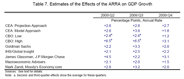
Table 7: from CEA, “The Economic Impact of the American Recovery and Reinvestment Act of 2009: Second Quarterly Report,” (January 13, 2009>.



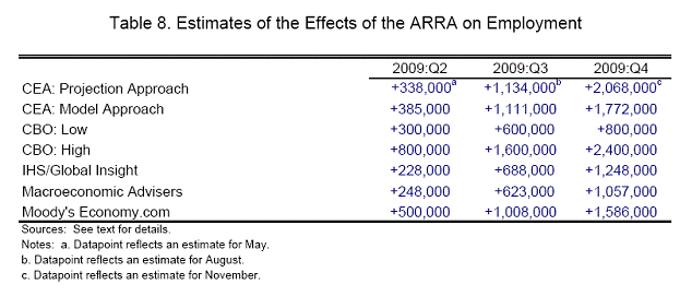
Table 8: from CEA, “The Economic Impact of the American Recovery and Reinvestment Act of 2009: Second Quarterly Report,” (January 13, 2009>.

Of course, the above set of models is not exhaustive, and John Taylor has argued for a broader set of models. I agree it would be useful to see for instance approaches, like the IMF’s GIMF DSGE, Davig and Leeper, as well as that of Christiano, Eichenbaum and Rebello, as discussed in this post. While the models cited by Taylor imply much smaller multipliers, the Laxton, the Davig and Leeper, as well as Christiano et al. models imply larger multipliers. (And of course, one should refer to Robert Hall’s recent paper on multipliers presented at the Fall Brookings Panel on Economic Activity.)

Turning specifically to methodology, I thought it of interest to look more closely at what the CEA calls its projection approach. They write:

There are many ways to construct a statistical baseline forecast. The particular method that we use is to estimate a vector autoregression (or VAR) using the logarithms of real GDP (in billions of chained 2005 dollars) and employment (in thousands, in the final month of the quarter) over the period 1990:Q1-2007:Q4. We include four lags of each variable. Because the estimation ends in 2007:Q4, the coefficient estimates used in the prediction are not influenced by developments in the current recession. Rather, they show the usual joint short-run dynamics of the two series over an extended sample. We then forecast GDP and employment in the second, third, and fourth quarters of 2009 using actual data through the first quarter of the year. Data through the first quarter include the monetary response to the current crisis, but not the fiscal stimulus or other actions that took effect after the first quarter. We have experimented with a variety of other ways of projecting the no-stimulus path of GDP and employment. The results of those exercises are similar to those we report below.

I have to say that the study is quite transparent in terms of the methodology; replication should be required for all the people who critique studies like this (and the journalists who report on them), so that they can then identify specifically where they disagree with a study. I easily replicated their analysis, and obtain the following graphs which show real GDP and end-of-quarter nonfarm payroll employment (both in logs). Note, in line with the CEA report, I use the 2009Q4 GDP Blue Chip forecasted increase of 4% (q/q, SAAR) to generate the 2009Q4 level of GDP. So in the case of GDP, output is 1.95% above baseline and NFP is 1.59% (both in log terms).

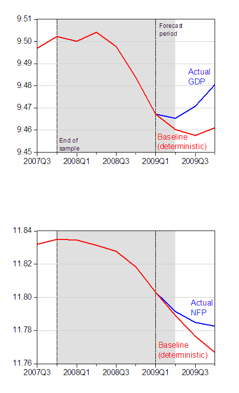
Figure 1: Log GDP [in billions of Ch.2005$] and log nonfarm payroll employment (NFP) baselines derived from deterministic dynamic simulation (red), and actual (blue). Gray shaded area denotes NBER recession dates, assuming trough at 2009M06. Source: BEA, BLS, and author’s calculations.

The results seem robust to moderate changes in the sample; expanding the sample backward to 1986Q1 (to more fully encompass the “Great Moderation” period) leads to 1.97% and 1.39%, respectively. In other words, the GDP impact is roughly the same, while the NFP impact is substantially larger.

I thought it of interest, though, to consider whether the difference is of statistical significance. So, I generate new baselines; in each case the baselines are the mean of the dynamically simulated forecasts, for 10,000 replications. In addition, I show the 50% confidence bounds, using bootstrapped innovations.

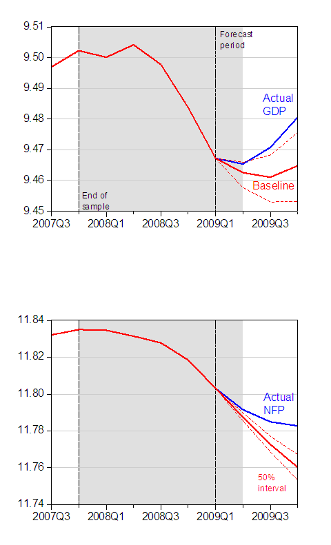
Figure 2: Log GDP [in billions of Ch.2005$] and log nonfarm payroll employment (NFP) baselines derived from stochastic dynamic simulation (red), and actual (blue). Bootstrapped 50% confidence bounds (10,000 replications). Gray shaded area denotes NBER recession dates, assuming trough at 2009M06. Source: BEA, BLS, and author’s calculations.

Interestingly, the mean of the stochastic simulations implies that output is only 1.59% above baseline, while employment is 2.25% above baseline. In both cases, economic activity is above what would be expected on the basis of random chance (with 50% confidence, which is admittedly below the conventional levels used, but is not that far away from what is standard in the VAR literature). Employment is, in this case, 2.92 million above baseline, rather than the 2.07 million found in the CEA analysis.

The key deficiency of this “projection” approach is that the difference between predicted and actual is a composite of the (potentially offsetting) effects of all the policies undertaken (monetary policy, regulatory policy, non-ARRA fiscal policy, as well as ARRA) as well as other events (rest-of-world GDP collapse, credit crunch). This argues for the model based approach I’ve discussed here.

On a separate note, I see some people have focused on the fact that the household survey indicates continued and substantial net job losses, as shown in this post. I include this graph of the volatility of the NFP and civilian employment series, measured as the log first difference of each series, to highlight the fact that the NFP exhibits substantially lower volatility than the civilian employment series.

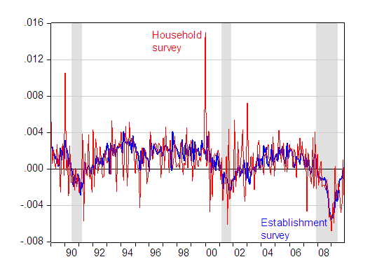
Figure 3: First difference of log nonfarm payroll employment (blue) and of civilian employment (red). NBER defined recession dates shaded gray, assumes last recession ended 2009M06. Source: BLS via FREDII.