In the wake of St. Louis Fed President James Bullard’s statement on the output gap [0] (which I frankly did not understand), there was renewed debate over output gap measurement [Duy] [Thoma] [Krugman]. I thought this was a good time to recap and update some of the material I’d written on this subject of output gaps.

DSGEs, Detrending, and Forecasting the Output Level

As somebody who has served on many dissertation committees where the dissertation involves cutting edge DSGEs (dynamic stochastic general equilibrium models), I can attest to the fact that such models can be very useful in providing insights into the workings of the macroeconomy, as well as the welfare implications associated differing policy regimes.

However, I think the observation that DSGE’s are at the cutting edge of academic research highlights several misconceptions, and one important drawback of DSGEs. (An excellent review of the use of DSGEs in policy is provided by C. Tovar)

Misconceptions

Regarding the treatment of expectations, DSGEs usually incorporate model consistent expectations. However, ever since John Taylor’s pathbreaking work in the early 1990s [0], we have had model-consistent expectations imbedded in certain structural macroeconometric models. Hence, a DSGE is not necessary for operationalizing rational expectations.

Regarding microfoundations, if one examines the guts of the standard New Keynesian versions (including the one recently used by John Taylor [1]), one usually finds lots of ad hoc additions. Consumption is definitely not described by a simple Euler equation as implied by the pure rational expectations-life cycle hypothesis; usually there are some hand-to-mouth consumers floating around. Prices are not freely flexible; rather Calvo pricing is often assumed for tractability. Capital adjustment costs, and other frictions are often included as well. Why not leave these frictions out? Because, without them, it is well nigh impossible to replicate the impulse response functions of real world data. In other words, the bright line of microfoundations versus ad hoc functions is in fact pretty fuzzy.

(And from an international finance perspective, it’s troubling that the real exchange rate is usually linked one-for-one with the ratio of the marginal utilities of consumption, something that is as counterfactual as one can get. And don’t get me started on the risk premium gets introduced into these models, if indeed there is one.)

The Big Drawback

DSGEs (and their predecessors, RBCs) are models of the business cycle. As such, they focus on the deviations from trend. However, in order to predict where the economy will be in one year, given current conditions and policies, one needs to know what the trend is. In other words, extracting the cycle from the trend is critically important. This is a point that James Morley made in his “Emperor has no clothes” paper.

This issue has long been recognized in the policy community. From Camilo Tovar:

Econometricians often fail to be able to observe the theoretical concepts modeled (eg the output
gap). So a first question is: how to match the theoretical concepts in DSGE models with those of
the observed data? This is not trivial (and certainly the problem is not exclusive to these models).
In the DSGE literature the theoretical concepts have been captured not against specific data
figures (say GDP levels or inflation) but against filtered data (eg by using the Hodrick-Prescott
filter). Filtering decomposes the data into a cyclical component and a trend component. The
cyclical component is what is frequently fed into the model. By doing so the analysis focuses
on the business cycle frequencies, mainly because it is considered that DSGE models are
better suited to explain short-run rather than long-run cycles. However, filtering has important
implications (see discussion in Del Negro and Schorfheide (2003)). One is that, forecasting
stays out of the reach of DSGE models since the goal is to forecast actual rather than filtered
data. The second is that the dynamics obtained do not match those required by policy makers,
weakening the usefulness of DSGE models as policy tools. Alternatives often used are the
linear detrending and demeaning of variables, as well, as transforming variables so that they
are stationary around a balanced growth path. In this last case, the problem is that the trend is
often assumed to follow an exogenous stochastic process, which is imposed by the researcher.

In order to highlight the real-world complications involved in this issue, consider two popular cycle-trend extraction methods used in the “business”: the Hodrick-Prescott (HP) filter, and band pass (BP) filter. I apply the HP and BP filters over the 1967Q1-11Q4 sample, and HP filter to the 1967Q1-09Q1 sample, and plot the resulting cycle components in Figure 1.

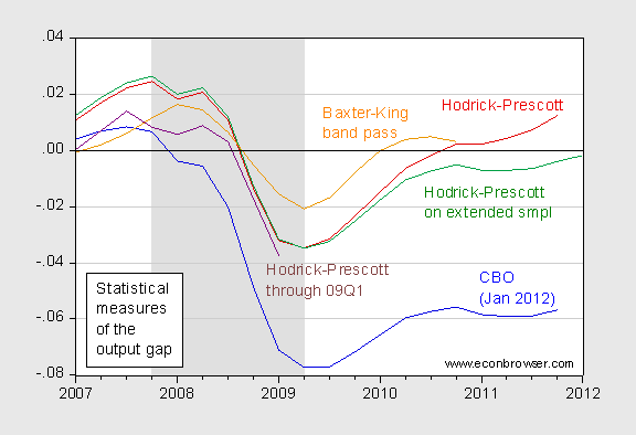
Figure 1: Log deviation from CBO measure of potential GDP (blue), log deviation from trend GDP, obtained using HP filter over entire sample, lambda=1600, estimated over 1967Q1-2011Q4 (dark red), using HP filter over sample extended 8 quarters (green), over sample ending 2009Q1 (purple), band pass filter with Baxter-King symmetric fixed length = 4 qtrs (orange). NBER defined recession dates shaded gray. Source: BEA 2011Q4 advance release, CBO, Budget and Economic Outlook (Jan 2012) supplemental data, NBER, and author’s calculations.

In order to mitigate the end-point problem associated with using a two-sided filter like the Hodrick-Prescott filter, the log GDP series are extended 8 quarters using an ARIMA(1,1,1), and then the filter applied (green line).

Figure 1 demonstrates how the inferences regarding the output gap differ wildly depending on the filter used; and the sensitivity of the results — even for a given filter — to the endpoints (notice how the HP filter gives different output gaps for 2009Q1 depending on the sample).

Appealing to simple theories does not necessarily yield uncontroversial results. In Figure 2, I plot the gap implied if one thinks GDP and consumption (here services only) are cointegrated. That approach, outlined by Cogley and Schaan (1995) following Cochrane (1994), implies that the economy was 2.7% above trend in 2011Q4.

For comparison, I include the CBO’s estimate from January 2012. Large scale macroeconometric models usually rely upon some sort of production function approach to calculating the trend. The implied output gaps from the consumption-cointegration approach and the CBO’s version of the production function approach (described here) are displayed in Figure 2.

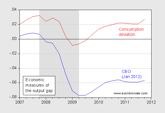
Figure 2: Log deviation from trend GDP, obtained using Engle-Granger cointegrating regression between log services consumption and log GDP (red), and log deviation from CBO’s potential GDP, January 2011 version (blue). NBER defined recession dates shaded gray. Source: BEA 2011Q4 advance release, CBO, Budget and Economic Outlook (Jan 2012) supplemental data, NBER, and author’s calculations.

For more on the scary things the HP filter can do, see T. Cogley, and J. Nason, 1995, “Effects of the Hodrick-Prescott filter on trend and difference stationary time series Implications for business cycle research,” Journal of Economic Dynamics and Control 19(1-2): 253-278. See also Simon van Norden on the use of these types of filters in current analysis. And for an excellent, albeit technical, exposition of the issues Gorodnichenko and Ng.

What Is It We Are Trying to Measure?

In his response to Duy, Bullard appeals to New Keynesian and two sector models of natural output and gaps, in a St. Louis Fed symposium on potential output (see this post for a discussion of the papers).

I found insights into this debate in this 2010 paper by Michael Kiley. From the paper:

What is the output gap? There are many definitions in the economics literature, all of which have a long history. I discuss three alternatives: the deviation of output from its long-run stochastic trend (i.e., the “Beveridge-Nelson cycle”);
the deviation of output from the level consistent with current technologies and
normal utilization of capital and labor input (i.e., the “production-function
approach”); and the deviation of output from “flexible-price” output (i.e., its
“natural rate”). Estimates of each concept are presented from a dynamic-
stochastic-general-equilibrium (DSGE) model of the U.S. economy used at the
Federal Reserve Board. Four points are emphasized: The DSGE model’s es
timate of the Beveridge-Nelson gap is very similar to gaps from policy institutions, but the DSGE model’s estimate of potential growth has a higher
variance and substantially different covariance with GDP growth; the natural
rate concept depends strongly on model assumptions and is not designed to
guide nominal interest rate movements in “Taylor” rules in the same way as
the other measures; the natural rate and production function trends converge to
the Beveridge-Nelson trend; and the DSGE model’s estimate of the Beveridge-
Nelson gap is as closely related to unemployment fluctuations as those from
policy institutions and has more predictive ability for inflation.

The output gaps are shown in three graphs from the paper.

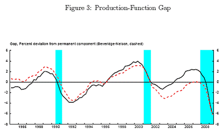
Figure 3 from Kiley (2010).



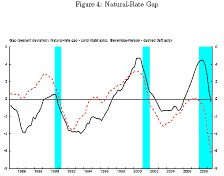
Figure 4 from Kiley (2010).



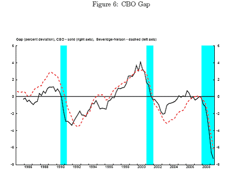
Figure 6 from Kiley (2010).

Based upon his analysis, Kiley makes the following four conclusions:

• The EDO model’s estimate of the output gap (according to either a Beveridge-Nelson or production-function approach) is very similar to gaps from the Congressional
  Budget Office or the Federal Reserve’s large-scale macro-econometric model (FRB/US) model, but the DSGE model’s estimate of potential growth is considerably more variable; the latter result stems from the significant degree of fluctuation in aggregate technology estimated by the DSGE model, a result consistent with the significant role such fluctuations play in model’s descended from those of the real-business-cycle tradition (from Kydland and Prescott (1982)).
  
• The flexible-price/natural-rate gaps are highly dependent on modeling assumptions,
  and their use in policy applications or forecasting requires a deep understanding
  of a specific model’s structure. (This result is closely related to the
  critique of DSGE models of Chari, Kehoe, and McGrattan (2009), who highlight
  the sensitivity of policy applications of such models to controversial modeling
  assumptions). In particular, a natural-rate gap does not provide the same type
  of guidance to a “Taylor” rule for nominal interest rates as other concepts of
  gaps; indeed, the signals from the Beveridge-Nelson gap provide a better sense
  of movements in the “natural rate of interest” than do the signals from the
  natural rate of output gap.
  
• “Equilibrium” or trend expected growth is highly variable in the flex-price/naturalrate
  case, implying that a focus on the current level of such gaps can be misleading
  in a policy discussion. In contrast, expected trend growth for the Beveridge-
  Nelson concept is exogenous and constant; moreover, all other notions of “trend”
  converge to the Beveridge-Nelson trend.
  
• The DSGE model’s estimate of the Beveridge-Nelson gap is as closely related to
  unemployment fluctuations as those from policy institutions (e.g., obeys Okun’s
  law) and has more predictive ability for inflation (e.g., has a tighter reduced form
  Phillips curve relationship).

For me, one important observation is that the output gap for both the production function based approach from EDO and the CBO estimate are of similar magnitude; 6 ppts and 7.5 ppts of GDP at 09Q2. The natural rate output gap is quite different, and this highlights the fact that this gap embodies a very different concept (discussed at length in the paper). I stress this, exactly because I know somebody is going to take some output gap measure and mis-interpret the implications of that gap — especially as concerns of inflation rise.

Concluding Thoughts

How do these observations relate to Bullard’s speculation? Here are my key take-aways:

• The observation that inflation has been higher than what is anticipated from traditional output gap measures is consistent with the natural rate output gap, rather than the deviation from potential GDP usually used. I wonder how a depeciating dollar and higher input prices fit into this story.
  
• Output gaps from DSGEs sometimes look different from production function based gaps (e.g., CBO), and sometimes don’t. It’s hard to generalize because there is considerable heterogeneity.
  
• When the DSGE output gaps are derived on series that have been detrended, one has to wonder abou the biases induced through the detrending process; it also complicates the forecasting of output levels, which is sometimes of primary interest.
  

A good review of issues is provided by the OECD.