Today, we are fortunate to have a guest contribution written by Laurent Ferrara (EconomiX-CNRS, University Paris West) and
and Valérie Mignon (EconomiX-CNRS, University Paris West and CEPII).
Following the recent financial crisis and its subsequent Great Recession, the issue of a sluggish US employment was raised by economic observers. In a previous post on Econbrowser, Menzie Chinn pointed out the usefulness of the Okun’s law in assessing the potential level of employment after the recession. Especially, Menzie shows that:
- If one does not account for the long-term relationship between GDP and employment (i.e.; if one focuses only on the relationship in differences), then the bounce-back in employment after the 2008-09 recession cannot be captured.
- A standard error-correction model (ECM) is able to reproduce the general evolutions, but misses a large part of the recovery after the end of the recession.
- Accounting for the US business cycle by incorporating a dummy variable that takes the value 1 during recessions and 0 otherwise, according to the NBER Dating Committee dating, enables a better reproduction of stylized facts.
In this work, we reconsider this ECM approach but we do not impose any dummy variable and propose to let the data speak through a non-linear ECM. More specifically, we retain the following non-linear specification:

where LEMP denotes private nonfarm payroll employment in logarithm, LGDP the logarithm of GDP, εt is iid, G denotes the transition function, γ is the slope parameter that determines the smoothness of the transition from one regime to the other, c is the threshold parameter, and Z denotes the transition variable.
This non-linear ECM takes the long-term relationship into account, as well as two regimes for the short-term relationship. More specifically, the economy can evolve in two states, but the transition between those two regimes is smooth: the two regimes are associated with large and small values of the transition variable relative to the threshold value, the switches from one regime to the other being governed by the transition variable Z. The smooth transition function, bounded between 0 and 1, takes a logistic form given by:
![]()
To account for the business cycle, we select as transition variable the average GDP growth over 2 quarters, lagged by 2 quarters, i.e.
![]()
We estimate this model over the period 1960q1 – 2007q4. The implementation of Johansen’s test leads to conclude to the existence of a cointegrating relationship between LEMP and LGDP. Once the estimation of this long-term relationship realized, we integrate the lagged residuals in our main non-linear equation.
The estimation of the non-linear specification is made following the methodology proposed by Teräsvirta (1994). We start by testing for the null hypothesis of linearity using the test introduced by Luukkonen et al. (1988). Once the null of linearity has been rejected, we select the specification of the transition function using the test sequence presented in Teräsvirta (1994). We refer for example to van Dijk, Teräsvirta and Franses (2002) for details on smooth transition models. We then estimate the non-linear ECM, leading to the results presented in the following table:
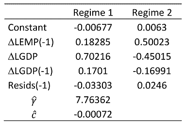
The estimated value cˆ of the threshold c is close to zero, delimiting thus periods of expansion and periods of recession, as shown by the transition function displayed in figure 1. The transition function is slightly lagged over the business cycle, underlining the point that the switch in regime intervenes at the end of the recession, or just after.
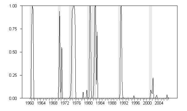
Figure 1: Estimated transition function and US recessions. Sources: authors’ calculations, and NBER for the dating of recessions. The gray bands represent US recessions.
This result confirms that the business cycle plays a non-negligible role in the short-term relationship between employment and output.
Second, we compute conditional dynamic forecasts of the variable LEMP over the period 2008q1 – 2012q3. This means that we forecast employment based on the knowledge of the ex post path for LGDP. The figure 2 below presents the observed employment (green line), as well conditional forecasts from a standard (linear) ECM (blue line) and from the non-linear ECM (red line).
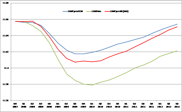
Figure 2: Conditional forecasts of employment (in logs) and observed employment (in logs). Source: Log private non-farm employment (green), conditional forecasts from standard error correction model (blue) and from non-linear error correction model (red), seasonally adjusted. Quarterly employment figures are average of monthly figures. Source BLS via FRED and authors’ calculations. Quarterly GDP data used to estimate the models are seasonally adjusted, expressed in billions of chained 2005 dollars. Source BEA via FRED.
We clearly see that both ECMs are able to reproduce the main movements in employment during and after the recession. However, there is a persistent gap between the observed employment (green line) and the conditional forecasts from both models (red and blue lines), meaning that the employment is currently well below what it should be according to the models. When comparing both ECM models, taking the non-linear business cycle into account through the non-linear ECM (red line) leads to reduction in the gap. But the contribution of the non-linear cycle to the employment is low (the difference between the blue and the red lines is around 1.2 % in 2010) and tends to diminish (the red line tends to the blue line).
This leads us to conclude that there has been indeed an effect of the Great Recession on the long-term employment. Specifically, on average, since the exit of the recession (2009q2), we get that the employment is 2.7 % below its potential level (according to the non-linear ECM), meaning that, from a structural point of view, around 3 millions of jobs have been lost after the recession. This interpretation is in line with the recent literature on this topic, as pointed out for example by Chen, Kannan, Loungani and Trehan (2011) or Stock and Watson (2012) that put forward various explanations.
Additional remark:
As in the linear framework, it is noteworthy that a non-linear model estimated in differences, that is without integrating a long-term relationship, also leads to unrealistic results. This underlines the usefulness of having the long-term relationship into the model.
Bibliography:
Luukkonen, R., Saikkonen, P. and Teräsvirta, T. (1988), Testing linearity against smooth transition autoregressive models, Biometrika 75, 491-499.
Teräsvirta, T. (1994), Specification, estimation, and evaluation of smooth transition autoregressive models, Journal of the American Statistical Association 89, 208-218.
This post written by Laurent Ferrara and
and Valérie Mignon.
I calculated a 2.84% jump in the natural rate of unemployment a couple of weeks ago using a much simpler equation.
unemployment = UT2 – labor share constraint + capacity utilization
labor share constraint is simply labor share (2005=100) – 22.6.
UT is a non-negative value for total unused available capacity for labor and capital.
7.7% = 0.9% – 71.6% + 78.4%
since 1967, the relationship between UT and unemployment moved along a curve with an equation of…
unemployment = 19.36×2 + 1.77x + 4.31
Since 1Q-2010, they have been moving along this curve…
unemployment = 6.62×2 + 6.11x + 7.15
The y-intercept determines the natural rate of unemployment. And we can see that the y-intercept has jumped up… 7.15 – 4.31 = 2.84%
Above they arrive at 2.7% and I arrive at 2.84%. Pretty much the same, yeah?
OK, so we’ve got a problem.
And what is the source of that problem? Not oil, is it?
Interesting conclusions.
So we’re to assume then that those 3 million jobs lost are permanent losses because observed employment is currently increasing at the same rate as the two ECM lines?
Furthermore, should we assume that observed employment will continue to remain parallel to the ECM curves as opposed to making a move towards it over the next couple of years?
Prof. Ferrara & Prof. Mignon Thanks. I’m assuming that the non-farm payroll and GDP data is seasonally adjusted? Your post didn’t specifically say.
I wonder about the asymmetric nature of non-farm payroll numbers. Some economists believe that during a recovery the non-farm payroll numbers from establishment surveys tend to underreport job growth because new companies (where much of the job growth might be coming from) are slow to make it on the BLS establishment survey. On the other hand, you might not see this difference between established firms and new firms at the downward swing of the business cycle. Could the lag in establishment payroll numbers account for some of the gap you are seeing? Something that might be corrected with longer lags perhaps?
Also, one of the things that makes the Great Recession different from your garden variety recession is the fact that we’re at the zero lower bound (ZLB). Obviously the ZLB represents a kind of policy threshold, so we might naturally expect an asymmetry in policy outcomes. What we directly observe is the nominal interest rate. What is of economic interest is the Wicksellian rate needed to clear markets, which was deeply negative during the Great Recession. Do you believe your threshold variable adequately accounts for the ZLB? In other words, might there be three regimes rather than just two regimes; viz., a “normal” regime, a “garden variety recession” regime, and a ZLB regime?
On raising the income bracket for tax increases:
At $400k+ income group, 8% of gross income = $90 bn; incremental tax bill of $32,000 for a $400k earner.
Relying only on $1 million+ earners: 8% of gross income = $60 bn.
Not enough, even after a vicious tax increase on the top brackets. That leaves only the lower brackets to close the gap later. Will the Democrats be willing to do that? There’s a huge policy risk for the Democrats in not taking a large, broad tax increase now. As Howard Dean has said, the fiscal cliff is likely to be the best deal the Democrats get.
And what’s happening to the AMT patch and the payroll tax holiday in all these negotiations?
Am I the only one who is getting the sense that Obama wants the cliff and is just looking to peg it on the Republians? Personally, I think the negotiating position of the Democrats come Jan. 1 is lousy. Working people are going to get hammered and are either going to blithely accept it or be screaming bloody murder for a deal with the Republicans.
The UT equation I show above is trending as a straight line towards the y-intercept “for now”, but it will start to curve upwards as more data comes in with UT closer to zero or even negative, which means that the natural rate of unemployment could bend higher than just 2.84% over the past trend. It could go be 3%+, but we need more data to pinpoint it.
Reply to Zeek… who said…
“…should we assume that observed employment will continue to remain parallel to the ECM curves as opposed to making a move towards it over the next couple of years?”
Yes… the economy does not have room to get back. The UT equation I use for this, also shows that potential GDP has fallen, better to say “backtracked” to a lower level. This means that growth is limited enough to keep this high natural rate of unemployment around for quite a while.
My UT equation shows that the real constraint on all this is low labor share of income. Once people start getting paid more on a long-term consistent basis, the economy will right itself.
u = UT2 + cu – W/Y
u = unemployment
UT = total available capacity for labor and capital
cu = capacity utilization
Wages = total wages
Y = real GDP, net income
Right now UT is close to zero, and labor share (W/Y) is lower. This means that for any level of capacity utilization, there is greater unemployment.
In the past, UT would have been larger at this point, allowing for lower unemployment.
If you raise the consistent trend of labor share of income, the natural rate of unemployment will trend back down.
To Edward’s point, look at the trend of reported labor productivity vs. wages, employment, private investment, and depreciation, and it is obvious that after-tax wages for the bottom 90% are not growing sufficiently fast enough, or at all, to imply faster consumption that would justify increasing production and capacity utilization.
We have replaced wage increases, which are said to be “inflationary”, with debt/asset inflation and concentrated returns from financial capital to the top 0.1-1% at the cost of compounding interest claims on all labor, profits, and gov’t receipts in perpetuity.
By the banksters printing trillions to bail out their balance sheets, they are encouraging further overvaluation of corporate equities to labor, investment, and GDP, which in turn maintains the incentive for hoarding savings at low-velocity exchange and non-productive speculative rentier activities.
Reply to Bruce…
In effect, you are right. institutionally labor share couldn’t possibly rise enough now. There isn’t enough time. Profit shares are already peaking macro-economically. We will have to go into an economic contraction first, which will “artificially” raise labor share.
The economy is broken. Eventually there will have to be a social movement representing your words of disgust…
Can you publish your estimated cointegration vector? I was not able to replicate your results with significant loading coefficients for the EC-term, i.e., the residuals from the first-stage regression of employment on GDP.
Accelerating automation and loss of employment and purchasing power for most of us in the next 5-10+ years will overwhelm policies that attempt to promote “job growth”, as well as render ineffective gov’t income support programs as tax receipts collapse:
http://ieet.org/index.php/IEET/more/pistono20121219
http://econfuture.wordpress.com/2012/12/04/robots-ai-and-automation-links/
Today, the Fortune 25-300 firms have total revenues equivalent to 100% of US private GDP at $425,000/employee; but these firms hire fewer than 13% of the US labor force, and they are the most likely to be able to afford to accelerate automation to scale, eliminating literally tens of millions of jobs in the US and worldwide.
The net energy per capita required to grow employment at an effective revenue or services per employee of $425,000 and more in the years ahead will not occur; therefore, the objective to encourage “growth” and “create jobs” is a futile objective.
What is instead required is “income and purchasing power” at the most efficient, least ecologically degrading, socially acceptable standard of material comfort and well-being at a sustainable exergetic equilibrium indefinitely.
We should be encouraging accelerating automation and elimination of jobs, replacing incomes, and reducing consumption, waste, and resource depletion in the process.
Today’s debt-based, financialized, global mass-consumer, oil- and auto-based model requiring infinite growth of population and resource consumption on a finite planet ain’t that.
Michael Hudson’s Reality Economics:
http://michael-hudson.com/2012/12/reality-economics/
. . . Finance has become the modern mode of warfare. It is cheaper to seize land by foreclosure rather than armed occupation, and to obtain rights to mineral wealth and public infrastructure by hooking governments and economies on debt than by invading them. Financial warfare aims at what military force did in times past, in a way that does not prompt subject populations to fight back – as long as they can be persuaded to accept the occupation as natural and even helpful. After indebting countries, creditors lobby to privatize natural monopolies and create new monopoly rights for themselves.
In the end we are led to hubris at the international level. Debts grow at an exponential rate (the Miracle of Compound Interest), making financial success all-absorbing – so much so that empires become self-defeating. That is the tragic flaw of high finance and military conquest alike.
Military overreach is what prompted aggressors to shift to financial modes of conquest. For economists who seek comfort in basing their discipline on physics, the relevant paradigm is Newton’s Third Law of Motion applied to international power politics: Every action creates an equal and opposite reaction. Exploited parties are impelled to break away – or become bankrupt.
The decay spreads from the imperial financial core itself as predators use their foreign financial booty to lord it over the population at home, polarizing and impoverishing the economy and thereby destroying the domestic market. That is the story of the decline and fall of the Roman Empire, and it should remain the standard economic model. Such a “market” is self-destructive.
or maybe there is no jobless recovery, but simply less jobs needed. Once debt servicing in the mortgage sector falls below debt production, I am sure a job surge will comes, but still be below past heights.
The only way you can expand jobs is through more demand, I mean a lot more demand. That is one of the points about ending the wage inflation push model for finance to take over.
In the 1930s and 1940s, when the modern system of national income and product accounts (NIPA) was being developed, the scope of national product was a hotly debated issue. No issue stirred more debate than the question, Should government product be included in gross product? Simon Kuznets (Nobel laureate in economic sciences, 1971), the most important American contributor to the development of the accounts, had major reservations about including all government purchases in national product. Over the years, others have elaborated on these reasons and adduced others.
Why should government product be excluded? First, the government’s activities may be viewed as giving rise to intermediate, rather than final products, even if the government provides such valuable services as enforcement of private property rights and settlement of disputes. Second, because most government services are not sold in markets, they have no market-determined prices to be used in calculating their total value to those who benefit from them. Third, because many government services arise from political, rather than economic motives and institutions, some of them may have little or no value. Indeed, some commentators—including the present writer—ultimately went so far as to assert that some government services have negative value: given a choice, the people victimized by these “services” would be willing to pay to be rid of them.
When the government attained massive proportions during World War II, this debate was set aside for the duration of the war, and the accounts were put into a form that best accommodated the government’s attempt to plan and control the economy for the primary purpose of winning the war. This situation of course dictated that the government’s spending, which grew to constitute almost half of the official GDP during the peak years of the war, be included in GDP, and the War Production Board, the Commerce Department, and other government agencies involved in calculating the NIPA recruited a large corps of clerks, accountants, economists, and others to carry out the work.
After the war, the Commerce Department, which carried forward the national accounting to which it had contributed during the war (since 1972 within its Bureau of Economic Analysis [BEA]), naturally preferred to continue the use of its favored system, which treats all government spending for final goods and services as part of GDP. Economists such as Kuznets, who did not favor this treatment, attempted for a while to continue their work along their own, different lines, but none of them could compete with the enormous, well-funded statistical organization the government possessed, and eventually almost all of them gave up and accepted the official NIPA.
Thus did government spending become lodged in the definition and measurement of GDP in a way that ensuing generations of economists, journalists, policy makers, and others considered appropriate and took for granted. Nonetheless, the issues that had been disputed at length in the 1930s and 1940s did not disappear. They were simply disregarded as if they had been resolved, even though they had not been resolved intellectually, but simply swept under the Commerce Department’s expansive (and expensive) rug. In particular, the inclusion of government spending in GDP remained extremely problematic.[Emphasis added]
– Robert Higgs, senior fellow in political economy for the Independent Institute and editor of The Independent Review
Ricardo There are many legitimate problems with the way NIPA accounts for GDP and NDP, but the ones you listed are hardly persuasive. For example, this claim:
because most government services are not sold in markets, they have no market-determined prices to be used in calculating their total value to those who benefit from them
First, even if you only included the private sector in GDP accounting, it is still not true that “total value” is used to compute GDP. GDP is based on the incremental value added at each stage of production. And the valuation reflects the extended market price of that incremental value, not “total value” under the demand curve. In other words, GDP does not account for consumer surplus, which would be part of “total value.” Except in the case of monopolies, in which case consumer surplus does get rolled into GDP. Indeed, this is one of the problems with much of the GDP growth in the 2000s…much of the growth in the financial sector was really just due to monopoly rents being picked up in productivity numbers. That quote also shows a deep misunderstanding about how the government evaluates the products and services that it provides. Government agencies actually work quite hard at estimating the market value of inputs and outputs. I urge you to compare the Lagrangian or “shadow price” or Hamiltonian models used by government agencies to the downright primitive models used in the private sector. Government agencies think very seriously about discount rates in a way that few private sector businesses ever do.
If you want to complain about NIPA accounting, then you should worry more about what doesn’t get counted than what does get counted. Household labor is not counted. The value of public goods is almost always understated because the true value is arrived at by vertical summation of benefit curves. And NDP does not properly account for the value of natural resources that are lost due to pollution, mining, tree harvesting, etc.
Slug,
Just because you work hard at solving a Sudoku puzzle doesn’t mean it has any economic meaning.
I have worked for a couple of major corporations for almost 45 years now. Every time I have asked suppliers to give me a comparison of the bid they make to us to a bid they make to government they laugh. The common answer is that they always bid higher to government because government invariably increases costs due to change orders and general incompetence. Governments have no way of using cost control mechanisms that are used by private businesses because they are non-competetive, political driven entities. Cost is secondary to the political implication. It is the nature of the beast.
“The common answer is that they always bid higher to government because government invariably increases costs due to change orders and general incompetence.”
I’ve also worked in a couple of Fortune 500 companies, and the way they commonly dealt with increased costs due to change orders and general incompetence was to stick it to the vendors using monies owed and future business as leverage. Maybe 2slugs can comment on the paradigm in the public sector.
Ricardo I think you missed my point. And your comment about vendors charging higher prices because of “change orders and general incompetence” actually contradicts your point that the government sector is immune to market discipline. Think about it.
In general the government faces the same input cost factors as the private sector. Compensation packages are roughly comparable over the business cycle. Government buys private sector goods & services at the market rate. Yes, there’s plenty of inefficiency in government, but I’ve worked for equally inefficient private sector firms as well. There are really two big problems peculiar to government expenditures. The first is that to a considerable extent the government has monopsony powers. For example, I work for DoD and we worry a lot about finding the right balance point between exercising monopsony power in order to save the taxpayer some money versus the suboptimal output associated with monopsony. On the other hand, a lot of DoD business involves monopoly sellers and the government as a monopsony buyer. So you have to negotiate a price. The second big difference is that government relies upon very sophisticated “shadow price” models to constrain budget submissions. These models correct for the tendency to ask for unlimited funds. For example, in the private sector the cutting edge multi-item multi-echelon MIME) inventory logistics model is some version of VARI-METRIC
http://or.journal.informs.org/content/34/2/311.abstract
Back in the mid-80s when the VARI-METRIC literature hit the journals it was already a decade behind where DoD was in MIME models.
In any event, nothing you’ve said supports your argument that government spending shouldn’t be included in GDP. You seem to think that higher prices due to inefficiency do not have any effect on the quantity of goods and services procured by government. And that is simply wrong.
Slug,
You can include anything you want to in GDP. My argument is not that government spending should not be included in GDP. My argument is that GDP is virtually meaningless because it is included. GDP only has meaning when it tells us about the health of the economy. If the government takes dollars and simply burns them but then records that as spending does it really tell us anything about the health of the economy. Use GDP all you want to, just don’t pretend it has any meaning.
Ricardo If the government takes dollars and simply burns them but then records that as spending does it really tell us anything about the health of the economy.
This statement reveals your ignorance about what “spending” means in the NIPA tables. If you want to criticize the way BEA computes GDP, then fine, but first try to understand just how it is computed. In your pithy example the only “product” in GDP would be the economic value of the heat coming from the bonfire of greenbacks.