And Implications for Current Macro Policy
In most of my discussions of macroeconomic policy, I have usually resorted to the textbook neoclassical synthesis, which assumes Keynesian behavior in the short run (nominal and real rigidities) and Classical behavior in the long run. Output then can go above or below potential (unemployment below or above the NAIRU) with symmetric response of price level or inflation. This worldview is not the only one; Paul Krugman has just noted one reason for asymmetries. Others have also noted related asymmetries, with resulting policy implications — including, Larry Summers and Janet Yellen.
In Summers and Delong (1988), the authors provide an interpretation of potential as a level of output that can’t be exceeded (to me this is reminiscent of the Friedman “plucking model” (re-iterated in a 1993 publication, see also [1], [2])). Figure 5 depicts per capita potential under this interpretation.
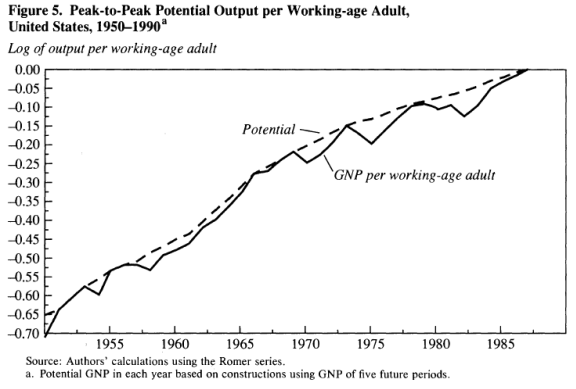
Figure 5 from Summers and Delong (1988).
The formula used is given by recursive application of their equation 17:
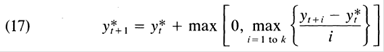
Where y* is potential GDP, and k=3 to 5. It’s of interest to consider what an updated version of the De Long-Summers procedure implies for the output gap. I apply the procedure to log GDP instead of per working age worker, and set k=3.
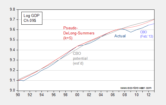
Figure 1: Log GDP (dark blue), CBO February 2013 projection (light blue), CBO potential, estimated by using 2011 ratio of 2009$ GDP to 2005$ GDP (gray), pseudo-DeLong-Summers (k=5) using actual data (dark red), and projection using CBO projections (pink). Source: BEA, CBO Budget and Economic Outlook (February 2013), and author’s calculations. [DeLong-Summers series calculation corrected 4:10pm]
As of 2012, the output gap using the DeLong-Summers (1988) procedure is quite similar to the implied CBO gap — 3.1% vs. 4.3% (log terms). There are a couple of caveats.
First, the CBO has not released an estimate of potential that is consistent with the newly back-revised BEA GDP series. Hence, I have resorted to the expedient of adjusting the CBO potential GDP series by the ratio of actual GDP in 2011, expressed in 2009$ and 2005$ from the respective series.
Second, since the calculation of the DeLong-Summers procedure requires values of future growth, one can only calculate the 2012 value using estimates of 2013, 2014 and 2015 growth. In the figure above, I use the CBO’s February 2013 projections. The upward movement in the potential GDP in 2013 (and later, not shown) is due to the projected surge in GDP growth in 2015 and 2016 (in excess of 4%). If one were to forecast tepid growth in those years, the trajectory of the pink line would be depressed with a commensurately smaller output gap, in absolute value. (Setting k=4 or k=3 would also yield a different set of estimates.)
So, the implied degree of policy activism one should pursue in 2013 could differ substantially depending on views of the evolution of potential. Note that in Delong and Summers (2012), potential is endogenous, depending on the level of current economic activity (hysteresis effects, etc.), providing an additional reason for pursuing activist macroeconomic (specifically, fiscal) policies.
The foregoing applies to thinking about long run aggregate supply. One can also think about short run aggregate supply, and relatedly, the Phillips Curve. In Yellen and Akerlof (2006), the authors note that the Phillips curve can exhibit marked nonlinearity, so a decrease in unemployment above NAIRU has a different size impact (in absolute value) than an increase in unemployment below NAIRU (For related discussion, see [3]). However, nonlinearity of this sort is not sufficient to explain the failure of inflation to fall during large negative output gaps.
They also trace out the possibility that at low inflation rates, the accelerationist hypothesis does not hold. In other words, the sum of lagged inflation rates do not determine current expected inflation. This interpretation is consistent with the experience during the Great Depression, and more recent experiences during the 1990’s.
From Yellen and Akerlof:
… Figure 4 presents data on the behavior of inflation for a number of OECD countries that experienced periods of prolonged unemployment in excess of their respectively estimated NAIRUs during the 1990s. The figure relies on OECD data and covers periods in which unemployment exceeded OECD estimates of the NAIRU. These recessions occurred in normal times, in the absence of an international gold standard. Most of the countries operated under a flexible exchange rate regime. The solid line shows the annual rate of inflation in the core CPI, while the bars again give the cumulative (n-period) change in inflation from an initial period in which unemployment exceeds NAIRU.
The behavior of inflation, as measured by the change in the core CPI since the beginning of the respective downturn, is again largely inconsistent with the adaptive expectations accelerationist hypothesis. …
(Note that this conclusion implies the estimated potential series in this post is not correct, at least for the years in which inflation is particularly low.)
This means in low-output, low-inflation environments, one should not expect marked increases in inflation for given increases in policy stimulus.
Summary
There are several ways of interpreting potential GDP, and hence the consequent size of the output gap. In this discussion I have eschewed discussion primarily statistical measures (HP, BP filters, discussed here) in favor of conceptual issues. In both cases, conceptions of how aggregate supply works imply activist macroeconomic policy is called for in current conditions, more so than in the case using a conventional, textbook AD-AS framework, even with large negative output gap, although the specific reasons differ.
At last, a pedagogic and not demagogic post from menzie chinn.
Concerned Citizens Brigade: Wow – this from the person who wrote (as John Locke) “Liberalism is a mental illness.” Hard to figure out how to take this compliment.
What exactly is an “activist macroeconomic policy?”
“There are several ways of interpreting potential GDP, and hence the consequent size of the output gap.”
Aren’t you assuming real AD is unlimited? If so, what if it is not unlimited?
Aggregates still distort reality. Anyone who builds a house on the beach based on aggregate measures of the tides will ultimately pay a price.
Friedman’s “Plucking Model” by Roger Garrison
http://research.stlouisfed.org/fredgraph.png?g=lEM
https://app.box.com/s/urkg7lqju0xz348shf2p
US real GDP per capita cannot grow with the price of oil above $40.
http://ycharts.com/indicators/us_household_formation
http://www.auction.com/blog/household-formations-have-slowed-considerably/
Household formation has plunged below the population growth rate and is again exhibiting implications for recessionary conditions for housing hereafter. The vast majority of young Americans age 35 and younger are in no position with respect to household finances, employment quality and tenure, income, purchasing power, and creditworthiness to couple and become mortgage debtors.
What economists are missing is the once-in-history structural shift in the composition of household spending from high-multiplier expenditures for housing, autos, and child rearing to low- or no-multiplier outlays for house maintenance, utilities, insurance premia, and out-of-pocket costs for medical services and medications.
Moreover, with unprecedented total public and private debt to wages, GDP, and gov’t receipts (coincident with EXTREME wealth and income concentration to the top 0.1-1% to 10% of households), there is no capacity to increase incrementally real GDP per capita growth from gov’t deficit spending. Low- or no-multiplier subsistence transfers, including food stamps and unemployment payments, do not add to the capital stock and growth of incremental demand and private production, employment, wages, incomes, and purchasing power.
Additionally, rapid growth of China-Asia’s consumption of energy and materials, resulting from US and Japanese firms’ large FDI growth since the ’90s, is the principal cause of the high price of oil and gasoline (coinciding with peak global crude oil production and falling production and oil exports per capita since ’05), which is constraining US real GDP per capita activity.
But in order for extraction of deep, tight, and tar oil to be profitable, the price of oil must be $85-$100+. The US cannot have growth of profitable extraction of costlier, lower-quality crude oil substitutes AND grow real GDP per capita, which is a condition characteristic of Peak Oil and the so-called “Seneca cliff”.
With unprecedented debt/GDP, OBSCENE wealth and income concentration to the top 1-10%, offshoring to China-Asia, $100-$110 oil, and the once-in-history Boomer demographic drag effects lasting into the ’30s, potential real US GDP per capita is 0%, or negative with growth of immigration.
I’d love to see a comparison of polling about expected inflation – not of economists – against the OECD numbers of what happens.
Menzie, he is right. Neo-liberalism is a mental disease.