Today we are fortunate to have a guest contribution by Ron Alquist, Policy Adviser at the Bank of Canada, and Olivier Coibion, Assistant Professor at the University of Texas, Austin. The views expressed here are those of the authors and should not be interpreted as representing the views of the Bank of Canada or any other institution with which the authors are affiliated.

From droughts in the American Midwest to labor strikes in the mines of South America to geopolitical instability in the Middle East, there are many potential sources of exogenous commodity-price fluctuations. Such changes in commodity prices can, in principle, have substantial macroeconomic effects and many have argued that shocks to commodity prices have indeed contributed significantly to global business cycles, such as those observed in the 1970s (Hamilton 1983; and Blinder and Rudd 2012) or more recently at the onset of the Great Recession (Hamilton 2009). But because commodity prices also respond to changes in global business cycle conditions, decomposing changes in commodity prices into those reflecting endogenous responses to global business cycles and those stemming from shocks originating in commodity markets has proven challenging. In a recent paper, we propose a new empirical strategy based on the theoretical predictions of a model of the comovement in non-energy commodity prices to identify the sources of historical commodity-price changes and their global macroeconomic implications (Alquist and Coibion 2014). The main conclusion of the paper is that commodity-related shocks have contributed modestly to global business cycle fluctuations, a finding in line with Kilian (2009) for oil markets.

Our approach to understanding the drivers of the comovement in commodity prices uses a theoretical model in which the prices of commodities are determined by two sets of forces. First, there are the forces that affect commodity prices directly, by which we mean forces which alter the supply or demand for commodities even for a fixed level of global economic activity. For example, we classify a technological improvement in the production of commodities as such a force, because it would increase the supply of commodities even in the absence of any subsequent effects on global economic activity. Of course, to the extent that these forces change commodity prices, they ultimately alter the level of global economic activity and feed back into commodity prices through general-equilibrium effects. But the key to identifying these forces is that they affect commodity prices even absent any endogenous response of global activity. By contrast, the second set of forces are those that affect commodity prices only through the changes that they induce in the level of global economic activity, i.e. “indirectly”. Changes in government spending, variation in the desired markups for the production of consumer goods, or improvements in the technology used to produce final goods are all examples of such forces. The composition of all such forces is summarized by the indirect factor. These two drivers are common to all commodity prices. The model also permits there to be idiosyncratic forces specific to individual commodities.

The key insight of classifying the common forces into these two categories is that they have different implications for the comovement in commodity prices. Specifically, the set of forces that affect commodity prices indirectly – that is, the indirect factor – through their effect on production all induce the same relative comovement in commodity prices, because their effects on commodity markets are summarized by their implications for global economic activity. Thus, for instance, an increase in the demand for commodities related to the global business cycle increases the prices of all commodities. By contrast, the common movement related to the forces that affect the supply of and demand for commodities directly – that is, the direct factor – induce different relative commodity-price movements. There is no guarantee that such changes induce similar comovement in commodity prices. Using the comovement of commodity prices therefore provides novel a way of identifying the channels underlying commodity price changes.

We apply these insights to a new data set of forty non-energy commodity prices to examine the role of these two factors in explaining historical commodity-price fluctuations. Figure 1 below depicts a historical decomposition of the annual percentage change in average commodity prices and relates them to the indirect and direct factors. The common driver that explains most of the variation in commodity prices is the one related to the indirect factor. Around 60 to 70% of the historical commodity-price movements are associated with the common driver that is related to aggregate non-commodity shocks rather than to direct shocks to commodity markets. During the commodity boom of 1973-74, for example, indirect shocks to commodity markets accounted for over two-thirds of the increase in commodity prices, with the remainder reflecting direct commodity-related shocks. Similarly, the fall in commodity prices during the Volcker era of the early 1980s is attributed almost entirely to a decrease in the indirect factor.

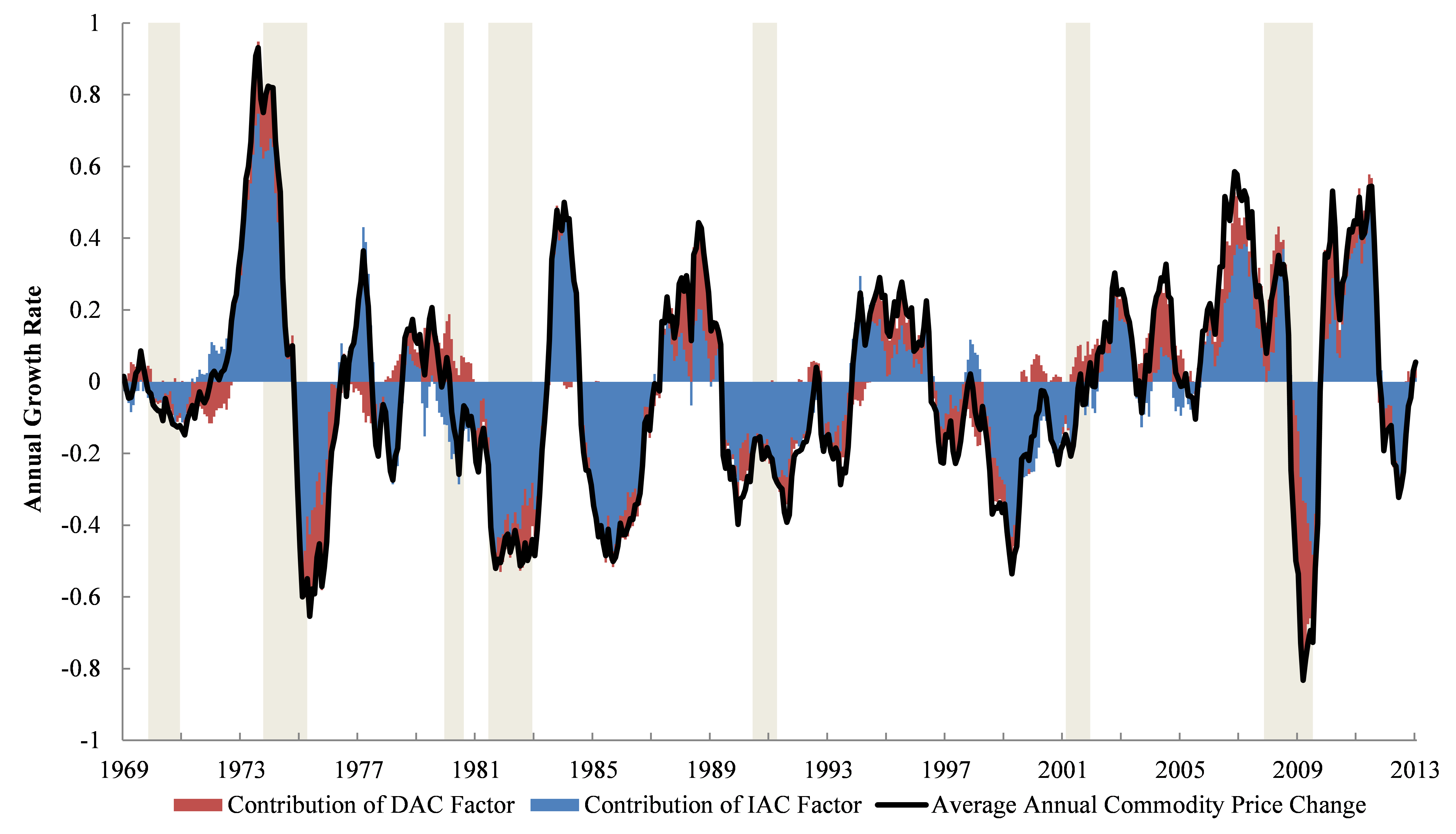
Figure 1: The Contribution of “Indirect” and “Direct” Factors to Historical Commodity-Price Changes. Notes: The figure plots the annual change in commodity prices (average across forty commodities): solid black line, the contribution coming from “indirect” global factors (IAC factor): blue shaded area, and the contribution from direct commodity factors (DAC factor): red shaded area. US recessions are identified using vertical grey shaded areas.

The second commodity boom of the 1970s, however, suggests a more nuanced interpretation. While the increase in commodity prices in 1976 reflected rising levels of global economic activity, the indirect factor contributed much less to rising commodity prices during the second half of 1978 and was actually pushing commodity prices lower for most of 1979. Despite this downward pressure from non-commodity shocks, the direct factor pushed real commodity prices higher during 1979 and did not weaken until early 1980. Thus, while the bulk of the second commodity boom of the 1970s can be interpreted as an endogenous response of commodity prices to non-commodity shocks, commodity-related shocks played an important role in extending the period of rising commodity prices into early 1980.

The decomposition of commodity prices since the early 2000s also presents a mixed interpretation. While a substantial share of the increase in commodity prices since 2003 is accounted for by the indirect factor, the direct factor accounts for much of the surge in prices during 2004 and about 30% of the increase from early 2006 to late 2007. The majority of the subsequent decrease in commodity prices between October of 2008 and March of 2009 is also attributable to the direct commodity factor, while the indirect factor accounts for most of the continuing decline after March 2009. Out of the total decline in commodity prices between October of 2008 and October of 2009, over half (56%) was due to direct commodity shocks. By contrast, the resurgence in commodity prices since the end of 2009 primarily reflects non-commodity shocks as measured by the indirect factor.

Our approach also has a more practical application: forecasting. Because we rely only on commodity prices traded on global markets, our decomposition can be applied in real-time to forecast a wide range of commodity prices within a common framework. We show that a simple model that includes the indirect factor and the price of an individual commodity generates out-of-sample improvements in forecast accuracy relative to the no-change forecast — that is, the forecast that assumes the price of the commodity does not change. The improvements in forecast accuracy are the largest at the 1- to 6-month horizons. What is more, the model helps to forecast the behavior of broader commodity-price indices, such as those produced by the IMF and the World Bank. The model also works well at forecasting the price of oil at short horizons. The improvements in oil forecasting accuracy are similar in size to those based on models of the global oil market (see, e.g., Baumeister and Kilian 2012; and Alquist et al. 2013), but our model does not require data on quantities produced, which are often available only with a delay. Our approach thus provides a coherent and tractable framework for forecasting commodity prices while also providing an economic interpretation for the forecasts.
In sum, our paper offers a new framework for identifying the sources and implications of commodity-price comovement and its relationship to global macroeconomic conditions. The framework provides an economic interpretation of the common factors driving commodity prices and offers a new perspective on the historical behavior of a broad cross-section of internationally traded commodities since the early 1970s. It can also be used to generate more accurate real-time forecasts for a wide range of commodity prices and commodity-price indices.

References

• Alquist, Ron and Olivier Coibion, 2014. “Commodity-Price Comovement and Global Economic Activity,” NBER Working Paper 20003.
  
• Alquist, Ron, Lutz Kilian, and Robert Vigfusson, 2013. “Forecasting the Price of Oil,” forthcoming in: G. Elliott and A. Timmermann (eds.), Handbook of Economic Forecasting, 2, Amsterdam: North-Holland.
  
• Baumeister, Christiane and Lutz Kilian, 2012. “Real-Time Forecasts of the Real Price of Oil,” Journal of Business and Economic Statistics, 30(2), 326-336.
  
• Blinder, Alan S. and Jeremy B. Rudd, 2012. “The Supply Shock Explanation of the Great Stagflation Revisited,” NBER Chapters, in: The Great Inflation: The Rebirth of Modern Central Banking National Bureau of Economic Research, Inc.
  
• Hamilton, James D., 1983. “Oil and the Macroeconomy since World War II,” Journal of Political Economy 91(2), 228-248.
  
• Hamilton, James D. 2009. “Causes and Consequences of the Oil Shock of 2007-2008,” Brookings Papers on Economic Activity 2009(2): 215-259.
  
• Kilian, Lutz. 2009. “Not All Oil Price Shocks Are Alike: Disentangling Demand and Supply Shocks in the Crude Oil Market,” American Economic Review, 99(3), June 2009, 1053-1069.

This post written by Ron Alquist and Olivier Coibion.