In my post on modeling the Kansas economy, Rick Stryker takes me to task for modeling the Palmer Drought Severity Index (PDSI) for Kansas as an I(1) process:
I wouldn’t bother with the ADF test, since its null is non-stationarity and it has low power to reject. I would focus on the KPSS, since its null of stationarity is almost certainly what’s really true.
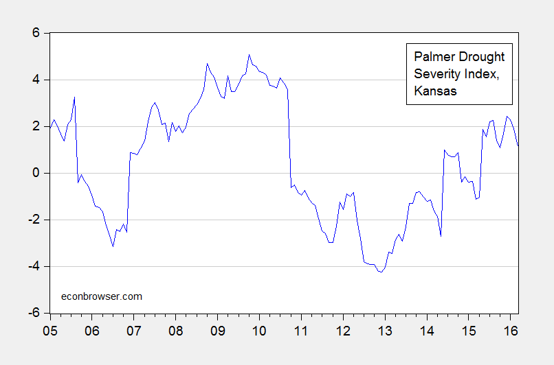
Figure 1: Palmer Drought Severity Index for Kansas. Source: NOAA.
Since proper accounting for unit roots is critical for obtaining proper inferences time series econometrics, I think it’s of some importance to highlight why taking the “Stryker view” is ill-advised. I turn to Dave Giles Econometrics Beat for support. From “Snakes in a Room”:
The other day my wife was in the room while I was on the ‘phone explaining to someone why we often like to apply BOTH the ADF test and the KPSS test when we’re trying to ascertain whether a partcular time-series is stationary or non-stationary. (More specifically, whether it is I(0) or I(1).) The conversation was, not surprisingly, relatively technical in nature.
… a useful analogy that one might use in this particular instance.
First, though, here’s a brief summary of the technical issue(s).
- We want to test if our time-series is I(1) or I(0).
- When we apply the ADF test the null hypothesis is that the series is I(1), while the alternative hypothesis is that it is I(0). On the other hand, the KPSS test is based on a null hypothesis that the series is I(0), and the alternative hypothesis is that it is I(1).
- So, the null and alternative hypotheses are reversed when we move from one test to the other.
- We also know that both of these tests can lack power in many situations. They’re not all that reliable.
- If we wrongly conclude that the series is I(0), when in fact it is I(1), this is pretty serious. We don’t want to end up working with a non-stationary time-series unwittingly. For instance, we may end up fittng a “spurious regression”.
- On the other hand, if we conclude that the series is I(1), when in fact it is I(0), this may not be quite so serious. For instance, if we were to (unnecessarily) difference the I(0) series it would still be stationary – although not I(0). That’s not so bad in itself, but it may mean that we don’t go on to test for possible cointegration between this series and any others that we may be working with.
- So, there’s a strong incentive to come to the correct conclusion when we test the data. For that reason, a “second opinion” might be a good idea. If both the ADF and KPSS tests lead us to the same conclusion, we might take some comfort from that.
Now, here’s my analogy. Suppose we have a dimly lit room with two windows, and in that room there are some snakes. They may be a completely harmless ones, or they may be deadly. Before entering the room, we’d like to try and figure what sort they are!
I take a flashlight, shine it in one window, and try to decide what I’m facing. I could go ahead on the basis of what I see through the one window using one flashlight and take a chance. Or, I could go around to the other window, perhaps use a different flashlight, and see what I can conclude from that different perspective.
If I come to the same conclusion about the nature of the snakes, whichever window and flashlight I use, then I may feel much better informed and prepared when I enter the room than if I come to diferent conclusions from the two viewings.
Wouldn’t you want to look through both windows before proceeding?
(For examples of looking through both windows, see Cheung and Chinn (Oxford Economic Papers, 1996), Cheung and Chinn (Journal of Business and Economic Statistics, 1997). Pay special attention to the bold face bullet points.
Over the 2005-2016Q1 period (used in the analysis), the Kansas PDSI fails to reject the unit root null in the Elliott-Rothenberg-Stock Dickey-Fuller test (constant, trend) at the 10% msl using EViews default settings/Bartlett window. It fails to reject the Kwiatkowski-Phillips-Schmidt-Shin trend stationary null at the 10% msl, using EViews default settings.
Interestingly, using monthly data, the KPSS test does reject at the 10% msl, but still fails to reject the ERS DF test at 10% msl.
So, for me, here are the takeaways:
- It’s best to treat most macro variables in levels (or log levels) as integrated.
- Just because a variable is by construction bounded does not mean that over the sample period it is best treated as stationary.
- Don’t make absolutist statements like “No, PDSI is clearly stationary as I’ve shown.”
Postscript: Rick Stryker also writes:
Because of the potential specification error problems, cointegration is not the first choice of many time series experts.
All I can say is, the term “many time series experts” reminds me of the phrase “some people believe” from the show “Ancient Aliens”. Sure, if all one is interested in is short run relationships, then first differenced data will obviate the need to deal with issues of cointegration. But if one wants to find the long run impact of money on the price level…
Hello,
This is so sad to hear, after all its end of the Year. Happy New Year..!!
Warm Regards,
Mathew
(http://www.ifsccodehub.com/)
Um ok. I reject both tests on purely logical grounds. The Palmer Drought severity test is, by definition, normalized to be between -10 and +10. https://climatedataguide.ucar.edu/climate-data/palmer-drought-severity-index-pdsi
It does take prior month conditions into account. But if it is bounded between +10 and -10 by construction, it cannot be I(1).
I do not know how much of Kansas GDP was affected by the drought. But if neither of you even understand how your drought severity index is constructed, I do not think either of you two do either.
dwb I’m not following you here. Yes, the PDSI is explicitly bounded, but as a practical matter I don’t see how that is significantly different than the implicitly bounded parameters we encounter in the real world. No one seriously believes that real world I(1) variables actually explode into infinity. You don’t seriously believe the S&P 500 is unbounded, do you? What we really care about is whether or not the variable tends to meander without any tendency to return to some mean within the sample range and likely out-of-sample range. And even if the variable is mean reverting, a very sluggish reversion is usually good enough to call it I(1). A phi value of 0.99 is (eventually) mean reverting, but I would highly recommend taking first differences. Besides, even if you over-difference you can always correct with some MA(q) term.
Time series analysis is not a substitute for knowing what your variables actually mean, how they are constructed, and what their limitations are. There is an actual answer, and it’s not found in a time series test. And no, very sluggish mean reversion is not “good enough” to call it I(1).
It did not take me long to dig it up in a few papers on PDSI either. Probably less time than spent debating whether to apply this or that time series test. See example here: http://journals.ametsoc.org/doi/pdf/10.1175/1520-0442(2004)017%3C2335%3AASPDSI%3E2.0.CO%3B2
Per the papers I dug up, monthly PDSI is by definition PDSI(i)= p* PDSI(i-1) + Z(i)/3, where Z is a moisture anomaly index. p =.897, typically (there are some complications during extreme drought or wetness). When the PDSI shows extreme drought or extreme wetness, the distribution is bi-modal because of switching. The paper I cited above suggests p should be determined regionally (and that the PDSI does not work well in the midwest), so with a little more digging I probably could track down the exact number if they are not using .897.
Worse that being misspecified in the regression, I now wonder whether the PDSI accurately captures drought conditions in the midwest. I still don’t know how much the drought impacted Kansas GDP. I am now pretty sure nobody else does either, and the answer cannot be found in a time series test.
Menzie,
You are omitting the nuance and context in making it sound like I proposed some sort of rule to use just one test for stationarity. I proposed no such thing as a look at my comment shows.
I agree with Giles’s view to use unit root tests with both nulls as a general practice, although context of what you are doing matters a lot. In my comment, I used both nulls in my analysis of the agricultural component of Kansas GDP for example, although I used the ERS rather than the ADF. I think you are missing the larger point of my comment. Just to restate it, my point was that it’s important to exercise judgment in how you do specification testing and to lay out exactly what choices you made and why you made them. If you have any additional information you can bring to bear, even if it is not formally statistical, I think it’s wise to use it. The results don’t just fall out of an econometric package as your post implied.
In the case of the PDSI, it still seems to me from the way the index is constructed and the underlying physics that it should be stationary, as we expect relative wetness and dryness to be mean reverting. But the more important problem I emphasized was the small sample we have–only 45 data points, implying potentially severe small sample bias in any test you run. Given the low power of the ADF I wouldn’t bother with it in this circumstance given my prior. Failure to reject would not influence my view very much. Of course, if I didn’t have a strong prior (and certainly if the sample size were larger), I would have looked at both tests. Instead, in this particular case it seemed much more important to me to focus on the KPSS test but be careful in specifying it in a way to handle the small sample bias. This isn’t easy, as there is a tradeoff between type 1 and type 2 error and it’s important to be clear how you think about that tradeoff. However, I showed that the KPSS results that confirmed stationarity were fairly robust to different tradeoffs of size and power.
You also missed the point of my comment that “Because of the potential specification error problems, cointegration is not the first choice of many time series experts.” I was not claiming in that comment that you should drop the cointegration term and just go with differences as you are implying. Nor is this a comment equivalent to saying that “some experts believe that we are visited by space aliens.” Rather, I was saying that cointegration is bedeviled with specification problems and there are alternatives.
Since you doubt my statement, allow me to quote from some experts then.
In John Cochrane’s lecture notes for his PhD time series econometrics notes at UChicago, he has this to say about cointegration on page 132: “There is much controversy over which approach is best. My opinion is that when you don’t really know whether there is cointegration or what the vector is, the AR in levels approach is probably better than the approach of a battery of tests for cointegration plus estimates of cointegrating relations followed by a companion or error correction VAR.”
In this well-known time series text that you may have heard of, the author in section 20.4 goes through the relative merits of ignoring non-stationarity and estimating a VAR in levels, differencing, or going through cointegration analysis. He says, “Experts differ in the advice offered for applied work.”
Ruey Tsay in his Analysis of Financial Time Series text also mentions the practical difficulties of using cointegration in practice. ‘
Happy New Year to you and econbrowser readers.