How to — and not do — time series analysis
Ironman of Political Calculations tries (and fails) to do a serious analysis of whether the drought had an impact on Kansas GDP. He fails on so many counts, it’s hard to cover all bases, but I’ll provide a few pointers. Overarching this entire debate, recall the initial question was whether the measured shortfall in Kansas overall GDP growth could be attributed to the drought.
Problem 1. Just because drought measurably affects the agricultural sector doesn’t mean the entire economy is measurably affected.
Agriculture, forestry, fishing, hunting (hereafter “agriculture”) value added has only accounted for on average 3.7% of Kansas GDP over the available sample period, as shown in Figure 1.
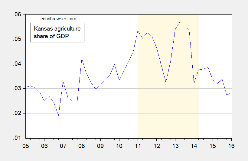
Figure 1: Share of Kansas GDP attributable to Agriculture, forestry, fishing, hunting (blue), and average value (red). Light brown shading is drought as defined by Political Calculations. Source: BEA (July 27, 2016), and author’s calculations.
I have no difficulty with the proposition that drought might have an impact on agricultural value added; but if agriculture only accounts for a small portion of the economy, one could have a drought and still not have a substantial impact on GDP.
Interestingly, the share of value added rises during the period Political Calculation alleges a drought induced hit to Kansas GDP. Expressing in real terms the (log) shares, one finds a similar story: the agriculture share is higher during the drought. (For a discussion of why log ratios are used, see here) This is shown in Figure 2.
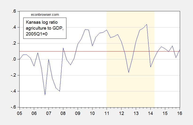
Figure 2: Log ratio of Kansas real GDP attributable to Agriculture, forestry, fishing, hunting minus log ratio in 2005Q1 (blue), and average value (red). Light brown shading is drought as defined by Political Calculations. Source: BEA (July 27, 2016), and author’s calculations.
If the drought so impacted agriculture so as to diminish Kansas GDP, why doesn’t it show up in these averages?
Problem 2. Running regressions when one doesn’t know what one is doing can be problematic. Ironman runs a simple bivariate regression of Kansas real agricultural output on the Kansas drought index. Nothing stops one from doing that; the question is whether the estimated coefficient converges in distribution to anything in particular. It won’t if both variables are stochastically trending, but fail to be cointegrated. Figure 3 shows the relevant time series.
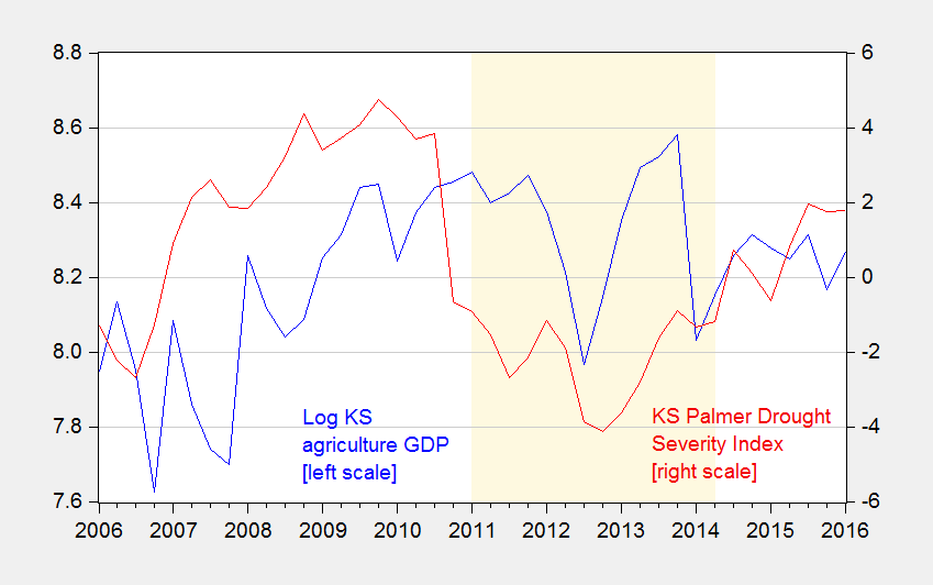
Figure 3: Kansas real GDP attributable to Agriculture, forestry, fishing, hunting, in millions Ch.2009$ (blue), and Palmer Drought Severity Index, PDSI (red). Light brown shading is drought as defined by Political Calculations. Source: BEA (July 27, 2016), NOAA, and author’s calculations. (graph updated to correct PDSI series for transcription errors, 9/11)
What do formal tests for stationarity indicate? For the level of real agricultural output Political Calculations uses, the Augmented Dickey Fuller test (constant, trend) fails to reject the null hypothesis of a unit root at the 5% level. The Kwiatkowski, Phillips, Schmidt, and Shin (KPSS) test with a trend stationarity null rejects at the 5% level (Bartlett kernel, Newey-West bandwidth). For more on the use of combination of unit root/trend stationary tests to make inferences, see e.g. Cheung and Chinn (Oxford Economic Papers, 1996).
What about the drought index? The level of this series fails to reject the unit root null at any conventional level of significance (5%, 10%, 20%, 50%). Depending on the specification, it fails to reject the trend stationary null at the 5% level (using Newey-West bandwidth, eviews default) or borderline rejects (using Andrews bandwidth).edited 9/12 So this too seems like an integrated series. So…if one had to guess, one could say both series are integrated of order 1.
In other words, Ironman is regressing an integrated series on an integrated series. The high R-squared (0.76) and big t-statistic (7.4) that Ironman touts is exactly what Granger and Newbold (1974) predicted when one regressed a random walk series on another random walk series, i.e., “spurious correlation”. Every serious empirical economist I know is aware of this; Ironman is apparently not. Unless the two series are cointegrated — a conventional Johansen maximum likelihood test, with constant in cointegrating vector, in test VAR, 1 lag of first differences fails to reject the no cointegration null hypothesis – estimation in first differences is then appropriate. (See this paper for a primer.) A simple regression of first (log) difference of agricultural output on the first difference of the drought index yields a regression result with a -0.01 -0.00 adjusted R-squared, and a t-statistic on the drought index of 1.05 1.44 (using HAC robust standard errors).
Problem 3. Forgetting the question. This debate arose because I asserted that lagging growth in Kansas economic activity overall was due to tax cuts and associated government spending cuts. Ironman asserted the drought was the culprit. But if one wants to answer the original question, one needs to look at what happened to Kansas GDP, not agricultural value added.
In order to find out what is attributable to what, one needs to include the factors deemed of importance. Hence, I estimate an error correction model incorporating (log) Kansas GDP, US GDP, the real value of the dollar for Kansas (from the Dallas Fed) in levels, and the Palmer Drought Severity Index (PDSI) and the government component of Kansas GDP in first differences. y is log GDP, r is the real value of the dollar for Kansas.
ΔytKS = 1.696 – 0.258 yt-1KS + 0.165 yt-1US -0.055rt-1 +0.993 Δ ytUS + (0 to 2 lags of first difference of PDSI) + (0 to 2 lags of first difference of log KS govt) + (0 to 2 lags of first difference of r)
Adj-R2 = 0.57, SER = 0.0077, n=41, sample = 2006q1-2016q1, Q(4) stat = 3.618[p-val = 0.451], Q(8) stat = 5.323[p-val = 0.723]. bold denotes significance at 5% msl, using HAC robust standard errors. bold italics denotes significance at 15% level. [Regression output] [Data] ]NOAA data, accessed 9/11/16] (PDSI data transcription errors corrected 9/11)
Real Kansas GDP and the fitted values from the estimated equation are displayed in Figure 4.

Figure 4: Kansas GDP in millions Ch.2009$ SAAR (blue), and fitted values (red). Left scale in log terms. Light brown shading is drought as defined by Political Calculations. Source: BEA (July 27, 2016), and author’s calculations (corrected 9/11).
A Wald test (F-test) for a restriction that the coefficients on the first differences of the dollar value are all zero fails to reject. The corresponding restriction for government value added is borderline rejected at the 5% level, and the restriction that the sum of the coefficients is zero is not rejected.
The joint restriction that all the coefficients on the PDSI are zero is also rejected. The interesting thing is that the only statistically significant coefficient goes the wrong direction: a worsening of the drought is associated with an acceleration in growth at a 2 quarter lag. In addition, the restriction the sum is zero is rejected, in favor of the alternative of a negative coefficient.
What variable is most important for determining the growth rate of the Kansas economy? The reported coefficients do not directly address that issue – that depends on the interaction of the coefficients and the independent variables. One way at getting at the question is to refer to a “standardized beta”. Of the statistically significant first difference terms, the largest is for contemporaneous US GDP; the second is government value added at lag 1 (0.32). The third is the PDSI at lag 2 (-0.22) – although the coefficient is of the opposite direction of what is asserted in Political Calculations.
Bottom line: Excel in the hands of the econometrically-ignorant is like a kid running with scissors.
Corollary: Government’s share of GDP in Kansas seems more important than the drought in driving Kansas growth rates.
Excel in the hands of the econometrically-ignorant is like a kid running with scissors.
Well, that’s sad but all too true. You at least spend most of your intellectual life in academia where folks are supposed to understand why you can’t regress non-stationary variables that don’t have a cointegrating relationship in order to keep the variables from wandering too far away from one another. But some of us have to suffer through briefings from management types that see trends and statistical relationships everywhere. And because Excel is ubiquitous the IT departments are convinced it’s the only software you need to analyze data. OTOH, I’m not sure we’d be any better off if Joe Schmoe started running regressions in EViews.
2slugbaits: I do tremble with fear thinking about what Ironman would do with EViews. But maybe just knowing the commands for “coint” and “uroot” exist, and the concepts of multiple regression and instrumental variables might give him pause for thought before trying to play statistician.
Professor Chinn,
I noticed that in EViews it seems to me that the same result is shown using dlog(x) and d(log(x)) and that if one uses paste special on a Word document after copying an EViews correlogram and clicking on “EViews Object” the result shows the bars in the original EViews correlogram as opposed to the ** notations. Is there a reason to use d(log(x)) rather than dlog(x) or am I miscalculating?
AS: I didn’t know you could type dlog(x) and that would give you the same results at d(log(x)). The only reason I can think of why doing it one way or the other is that if you want to forecast x, then better to put in d(log(x)). If for instance you generated y = d(log(x)) and ran a regression of y on something, and forecasted y, you’d get a forecast of d(log(x)) and not of x.
I notice that using the forecast function in EViews, the same forecast options are available whether one starts with dlog(x) or with d(log(x)). You can forecast either (x) or dlog(x) or (x) and d(log(x)). Since dlog(x) and d(log(x)) are the same, the forecast options are the same.
Please excuse if this double posts. The first post did not seem to go through.
AS: Good point — I do it the way I do so that I don’t have to click to change the option. But in EViews you can get whatever you want, pretty much.
I do things in a particular way out of inertia — I have been using EViews so long that when I started out, it was called MicroTSP, and nearly all commands had to be typed out.
I notice that when one uses the forecast button in EViews in either case the forecast can be for (x) or it can be for dlog(x) or for (X) and for d(log(x)) and since dlog(x) is the same as d(log(x)), the same forecast options are available in EViews, unless I misunderstand your comment.
AS: Not sure, as I usually type in the commands.
But consider the case of LS. Suppose you want to run a regression of log(Z) on log(V). You could use “ls log(Z) c log(V)”, or first generate lz = log(Z), lv = log(V), the use “ls lz c lv”. In EViews, if you then type “forcst”, the former will provide a forecast of Z, the latter, a forcast of lz. Which one you want will determine which way you do things.
I understand your example and have noticed from experience what you show. I wonder if you try using commands if the dlog(x) and d(log(x)) may give the same forecast options. Not being argumentative, just trying to better understand EViews and follow your models. I appreciate your examples with data and output. Great learning opportunities.
Professor Chinn,
You do a great service for anyone interested in proper presentation of data (amongst all your other posts). It would be very difficult for most folks to enjoy the enlightenment you offer without enrolling in economics courses. I am always perplexed about why economic blog authors don’t have an economics advisor to review comments to avoid making the type of errors you explain. Thanks for what you do. If an analysis fits with your blog topics, it would be great for an ARDL example using I(0) and I(1) data. Professor Giles presented a great example on his blog using the new Bounds test in EViews 9.5 and Long-Run characteristics or the ARDL model. Something that does not seem to be clear is the co-integration model in the ARDL model presented in EViews 9.5 as compared with an ECM model, since the ARDL model can have I(0) and (1) data.
Menzie,
I guess I learned two things from this post. First, Ironman is a member of the 99.999..% of the population that doesn’t have a PhD in economics with research interests involving time series econometrics. And second, you are never going to stop hating on Ironman. But on reflection, there is a third point that I’m not sure you intended.
Your point is that excel in the hands of the econometrically illiterate is like a kid running with scissors. If you had left it at that, I would have been fine with it. But when you suddenly discover by doing econometrics “correctly” that the relatively weaker growth in Kansas GDP is a result of Brownback’s policies, I realized that there is a deeper point: eviews in the hands of a man with an agenda can be just as dangerous.
The 99.999..% has no idea what you are talking about in this post. But if they waded through it at all, I think they are supposed to get the impression that if they know some the secret incantations of the economics guild, such as “KPSS test” or “Johansen method” and have powerful enough software, they can check a few option boxes and “Vote For Democrats in Kansas” will pop out like magic.
The 0.0..01% knows better. Cointegration methods are bedeviled with specification error problems. In Johansen, how you set up the form of the VECM matters. How you specify the constant terms matters. Often the multivariate trace and maximum eigenvalue tests disagree. The procedure is a multi-step process in which an error in one stage can pollute the results in the next. Small sample bias is a huge problem to deal with. It’s very easy to misspecify one of these regressions. Even if you do all this specification analysis and are satisfied, there is the rather huge leap in treating government spending as exogenous and causing Kansas GDP. This is a much bigger issue.
Because of the potential specification error problems, cointegration is not the first choice of many time series experts. It’s not necessarily the “correct” way. That’s not to say that no one ever should use it. If you do decide to use it, you just have to be pretty methodical and cautious, recognizing all the pitfalls. How you deal with causation in time series econometrics is a much thornier issue.
So, I guess I come to a different bottom line for the 99.999..%. Kids, don’t try this at home. Leave it to the professionals. The econometric software won’t tell you to vote against Brownback just because you checked the approved boxes in the econometric package using the “correct” econometric methods.
Rick Stryker: Let me make a few observations on your desperate attempt to vindicate Ironman’s approach to econometrics.
(1) When I taught econometrics at the Master’s level, I discussed integration/cointegration. Some 25 years after the advent of the Johansen approach, one would think this is something in the toolkit of empirical economists working with time series.
(2) My objective is not to conclude that Brownback was wrong. Rather, it was the more general point that if one is to try to prove that the drought induced overall economic activity to lag, then (2a) running a regression of integrated series on integrated series was a poor way of doing it, unless very special conditions (which don’t seem to hold) hold; (2b) that overall economic activity is the variable one should not be looking at, not a small component of overall economic activity.
(3) I understand the complications involved with using the Johansen ML approach; heck, I cite them in many of my papers — look ’em up if you don’t believe. But, for instance, you can’t find evidence of cointegration at the 5% msl using aysmptotic critical values for any of the usual specifications involving constants and trends, and one lag of first difference, equal to 2 lags in VAR specification, for real KS agricultural output and the Kansas Palmer drought index. And if you use finite sample critical vales, you’ll have even less luck. And if you add in more lags in the VECM, less, less luck.
So, keep on waving your hands to try to rescue Ironman. You embarrass nobody but yourself in your desperation.
Oh, by the way — I don’t hate Ironman. I actually kind of like him, because he gives me so many examples to use in econometrics classes and posts on econometrics (actually, just plain data use, as exampled in his messing up repeatedly with chain-weighted indices; he’ll make it into the year-end review multiple times this December!). (I must confess, I also pity him for his pure data-haplessness.)
Menzie,
I was trying to make a serious point but you’ve accused me of “waving my hands.” I guess I have to get to work then, on a Sunday morning no less. So, let me get more specific then about what I’m talking about.
First, before we can get anywhere, we have to make sure that we are all using the same data. I collected Ag Kansas GDP from the BEA as well as the Palmer Drought Severity Index (PDSI) from the NOAA and did some analysis. I don’t get the same results as you do. On the PDSI, part of the explanation may be that you don’t seem to be using the same data as Ironman. Compare your figure 3 with the third chart in Ironman’s post.. Your PDSI data is pretty dramatically different from his. The data I independently collected follows Ironman’s chart closely. To convert Ironman’s monthly data to quarterly, I averaged the data over the 3 months in each quarter.
One point I made earlier is that your post gives the impression that if you just check the right boxes in the software package, out falls the result. One point I was making is that in applied econometrics before checking the boxes you have to think carefully about the problem. For example, before we run any tests, what does the economics (or physics) of the problem tell us about whether a series is likely to be stationary or not? The PDSI is an index based on a formula to determine the degree of dryness. Since nature can get only so dry or wet, it must have an upper and lower bound. One source I saw said the PDSI is bounded between a standardized -10 and 10, although in practice the index never sees those extremes. A priori, then, the PDSI can’t be a unit root process, because there is no path on which it can wander off to some arbitrary value.
Just to confirm that, I wouldn’t bother with the ADF test, since its null is non-stationarity and it has low power to reject. I would focus on the KPSS, since its null of stationarity is almost certainly what’s really true. Because we have only 45 data points, we do have to worry about small sample bias. The KPSS test is oversized in small samples and there is of course a trade off between size and power. I don’t think we just want to let the software package automatically choose the bandwidth of the test.
Eviews seems to use the Bartlett Kernel with the Newey-West lag selection formula. I favor using the rule suggested by KPSS and Schwert, available in R, since we can directly compare to the monte carlo evidence reported in that paper. I’d use the longer lag length, an integer value of 12 in the lag length formula, since that keeps the size more correct and I’m more worried about size than power given my prior. I also specify the non-trending version of the test. When I run the KPSS test, I can’t reject the null at the 5 or 10% levels. That result is robust to using a shorter lag length as well–using 4 in the formula–in which the test will have more power in small samples. Thus, the KPSS test seems to confirm what we would expect, that the PDSI is stationary.
Turning to the AG component of Kansas GDP, I would think we need to run tests with both nulls, since I don’t have strong priors on whether the series is stationary or not. I would not use the ADF as you have, because of its poor power characteristics and tendency to call series non-stationary. For the null of non-stationarity, I would use the Elliot-Rothenberg-Stock test because of its optimal power characteristics.
ERS has two tests, a feasible point-optimal “P test” and a modified ADF-type test. I run the trend version of both tests. In the modified ADF-type test, I can’t reject the null of non-stationarity However, if I use the “P test,” I can reject the null at the 5% and 1%. So, the two versions of the test are giving conflicting results.
Turning to the KPSS test for the AG Kansas GDP, we have to consider the lag length to use. Since the test is oversized, using a longer lag length helps to correct that problem in samples this small. However, the power is reduced. Using a shorter lag length improves power at the expense of oversizing however. Since we are not sure, I’d run with both lag lengths. With the longer lag length, using 12 in the formula, I can’t reject the null at the 5% level. With the shorter lag length, I can reject the null at the 5% level. Thus, the KPSS is giving contradictory results too.
From my analysis, the jury seems to be out on whether the AG Kansas GDP is non-stationary. Ironman’s regression might be just fine from a spurious regression point of view, since he could be regressing stationary series on each other. Your point, it seems to me, that Ironman has estimated a spurious regression is wrong. In the worst case, he has regressed a stationary (PDSI) against a non-stationary variable (AG GDP), which is a fundamentally misspecified regression, since you can’t really do that. But that’s a very different problem.
My comment was also directed at an analysis you did, in which you estimated an error correction model. You didn’t spell out the details, but I assume you used Johansen to determine that the 3 variables were cointegrated, that there is only one cointegrating vector, etc. etc. to arrive at your specification. My point about that was that are many choices to make along the way, as above, and many ways to misspecify the model. If, for example, you put PDSI into the Johansen procedure with the other variables in the system and it’s really stationary, that will likely produce a specification error that goes into the next stage. I don’t know what you did here, but it’s a general point about cointegration methods. Also, I’d mention again that treating government spending as exogenous is quite a leap. It’s not an automatic process. You have to make some judgment calls as I did above. Reasonable people can differ on these calls of course.
There are alternatives to ECMs as I know you are aware, but the 99.99..% reading this (or not reading at this point more likely) won’t know about that. Some people favor a VAR in levels instead to avoid the specification error problems. Estimates are consistent and many hypothesis tests of interest are valid, although some have non-standard distributions. But I guess you give up efficiency. There is no easy answer.
From my point of view, there is only weak evidence that Ironman’s regression is problematic from a spurious regression point of view. It may well be just fine and so I don’t think the diatribe you have directed against him is justified. And no one should assume that the ECM you did is the last word because you did it “correctly.”
Rick Stryker: On the PDSI, I discovered a data transcription error last night, re-estimated and replotted and reposted as of 9pm (Pacific). Apologies if you did not see the updated post, and apologies to all for the error. The regression results and Excel spreadsheet are updated.
1. In this post, I did not mention Brownback once. The question was whether weather as summarized by PDSI was influential; it was not. With corrected data, it still isn’t.
2. I re-checked using Johansen (all conventional specs re: trends, constant), and found no evidence of cointegration agriculture with PDSI.
3. I agree the unit root test results are not definitive. But in my (admittedly intuitive) approach, if results pop out easily, it’s hard to dismiss. If you have to work to get e.g., stationarity, well, I’d worry.
4. PDSI must be stationary. I agree! But so too should the “great ratios” in macro, such as C/Y. Well, I can tell you it’s hard to reject a unit root even with long historical data. What does that tell you? In finite samples, you can get no-reject even when you know with infinite data you’d reject. (Of course, with infinite data, we’d always reject the unit root null!). So the question is how to best treat the data with the sample sizes given…
5. I concur treatment of government value added (in log first difference) as exogenous is important. Change lags from “0 to 2” to “1 to 3”. I can’t reject Wald tests for joint null, or summed value equals zero. Also can’t reject corresponding for weather as summarized by the Kansas PDSI.
Last point of curiosity: Ironman’s results are all for an old data vintage. I don’t have exactly that vintage, but with the most recent, many of those reported results fall apart. Ironman makes no mention of that point. I have a agriculture series that is close to same vintage as the one he uses; I sincerely doubt you’d reject the unit root null even using ERS.
5.
Menzie,
I saw that you changed it this morning. Yes, it looked like there was a problem yesterday more at the end of the chart but I didn’t look all that carefully. But the new data you have also looks problematic. Look at your 2007 Q1 value in your chart. You have something close to -1.1. Ironman in his chart has something close to or above +1. In Q1 2011, you have what looks to me to be about 1 in your chart. Ironman has around -1. In 2014 Q1, Ironman has around -1.3. You have a little less than 1.
I think there may still a problem with the PDSI data.
Rick Stryker: Thanks for pointing that out. I did make a mistake (I think I had retrieved state “10” instead of “14”), so I have updated yet again. Most of my results revert to what I had initially, which is more contra Ironman’s results.
I’ve added a link to the NOAA data, below the regression results, so you can cross-check I have the right data.
Menzie,
Now that the PDSI data is fixed, we can return to the question of its stationarity. As I pointed out, a apriori we’d expect that series to be stationary. When I ran the KPSS test, using the non-trending option, I cannot reject the null of stationarity, whether I use 12 or 4 as the integer in the bandwidth selection formula that KPSS recommend. You assert that you can reject the null at the 5% level, although you were not specific about the options you used in the test. I don’t see how that can happen. I checked the test using the Newey-West automatic procedure that I believe eviews uses and was not able to reject the null in that case either. The only way I can reject the null at the 5% level is if I set a very short bandwidth.
You seem to imply that you used the trend option in KPSS. That makes no sense since the PDSI is not a trending series. Nonetheless, even if I assume the trending option, I can’t reject the null using my two bandwidth selection options or the the Newey-West automatic procedure.
What assumptions did you make in the KPSS test?
Rick Stryker: Default options fails to reject at 10%, would guess reject at 15%. Try any AR spectral methods (which is default in ERS you used).
Menzie,
AR spectral methods are not the default in KPSS tests though.
Using any of the standard KPSS methods, the Palmer Drought Severity Index (PSDI) is very clearly stationary. As I mentioned, that result holds for the standard Bartlett kernel for a range of standard bandwidths. It also holds for the less standard but still used Parzen and Quadratic Spectral kernels. You used the standard Bartlett Kernel and standard Newey-West bandwidth for the KPSS test when you applied it to agricultural output. In the next section on the PDSI variable, you didn’t think it worth mentioning that using the standard assumptions the KPSS test pronounced the PDSI series stationary? Or mentioning that you had suddenly switched to a non-standard method? Or that that non-standard method was giving highly unbelievable results? Using the OLS autoregressive spectral density estimator and the Schwarz information criterion for bandwidth, the KPSS test statistic implies a very massive rejection of a null at very, very high confidence levels never seen in practice of a hypothesis that we know a priori to be true.
The evidence that the PDSI is stationary is strong. Therefore, Ironman did not estimate a spurious regression. Given the weakness of the evidence on the non-stationarity of Ag output, his regression may have been just fine. Moreover, the Johansen cointegration analysis you did to establish that AG output and PDSI are not cointegrated was not legitimate.
You told me in your comment above that “(y)ou embarrass nobody but yourself in your desperation.” I think you are that point now. You began your indictment of Ironman using incorrect data. Then, you followed up with new estimates using incorrect data. With the data finally corrected, there is no case. Isn’t it time to acknowledge that this post didn’t work out and move on?
Rick Stryker: I agree PDSI-KS could be stationary, but like I say, it fails to reject unit root using ADF (default), and would borderline reject KPSS (using default), which in my book is more consistent with nonstationarity than stationarity. (Did you note that if you use Andrews bandwidth, you reject KPSS null at 5%?)
But clearly agricultural output is nonstationary. If you get the vintage of agricultural output Ironman uses, you will see it is even less likely to be stationary than the one I use. So I respectfully submit, it was ill-advised for Ironman to ignore issues of stationarity.
I think you would agree, unless you think it’s just a wonderful idea to regress a clearly nonstationary series on a possibly stationary series, but equally likely nonstationary.
No, PDSI is clearly stationary as I’ve shown. From a theoretical point of view it must be stationary. Failure to reject the null in KPSS at standard confidence levels is a robust result across a range of standard kernels and standard bandwidths. You claimed above that you can reject KPSS at the 5% level in the post but you are now saying it would “borderline reject” even though you can’t reject at the 5% or the 10%. Don’t you want to correct the record in the post on that? Your reliance on the ADF test is ridiculous. There are 45 data points and that test has very low power in such small samples. Finally, you can reject at 5% with the Andrews bandwidth only if you make the assumption that PDSI is trending, which I’ve already noted is a false assumption for this series. If you don’t assume it’s trending, you comfortably fail to reject at both the 5% and 10% levels.
You’ve also just asserted that AG output is clear nonstationary but I’ve already shown that’s not true. The result is not robust to reasonable changes in the ERS or KPSS tests. It’s not clear if the AG output is stationary or not.
The conclusion stands. PDSI is stationary and we can’t be sure about AG output. Your results are illegitimate and you owe Ironman an apology. You are denying the obvious and illustrating the truth in my first comment, to wit: “Eviews in the hands of a man with an agenda can be just as dangerous.”
Rick Stryker: I’ve amended my text to account for the varying results. I’ve added a new post which addresses the relevance of the “a priori” condition for making inferences.
Professor Chinn,
Would you consider posting your EViews output for your unit root tests on PDSI? I think I am in sync with you two experts on KPSS but not on the ADF test. I am assuming that the PDSI column on the Excel link above for the NOAA worksheet is for KS. Thanks.
AS: I’ve posted the unit root test output, plus summary and graphs, here.
Thank you!
I wonder about Ironman’s rationale for using he PDSI. Setting aside the extreme autocorrelation in the data, there’s the larger issue about the appropriateness of the PDSI. Ironman’s hidden assumption is that agricultural output is negatively correlated with drought and positively correlated with moisture. He may not be aware of it, but that is the hidden assumption in his analysis. This is pretty clearly wrong. Too much moisture can be just as much of a problem as too little. So we wouldn’t expect a monotonic relationship between output and the signed values of the PDSI. Maybe with the absolute deviations, but not the signed deviations. You also have to check the month. Dry conditions shortly before harvest times are likely to increase output. So it’s not just that Ironman doesn’t understand time series econometrics, it sounds like he doesn’t understand agronomy either.