In a forthcoming paper (“The New Fama Puzzle”), coauthored with Matthieu Bussière (Banque de France), Laurent Ferrara (Banque de France), Jonas Heipertz (Paris School of Economics), we re-examine uncovered interest parity – the proposition that anticipated exchange rate changes should offset interest rate differentials. This is one of the most central concepts in international finance. At the same time, empirical validation of this concept has proven elusive. In fact, the failure of the joint hypothesis of uncovered interest rate parity (UIP) and rational expectations – sometimes termed the unbiasedness hypothesis – is one of the most robust empirical regularities in the literature. The most commonplace explanations – such as the existence of an exchange risk premium, which drives a wedge between forward rates and expected future spot rates – have little empirical verification.
Why Revisit?
Several developments have prompted this revisit. First and foremost, the last decade includes a period in which short rates have effectively hit the zero interest rate bound. This point is clearly illustrated in Figure 1 where we plot three-month interest rates for a set of eight selected countries. This development affords us the opportunity to examine whether the Fama puzzle is a general phenomenon or one that is regime-dependent.
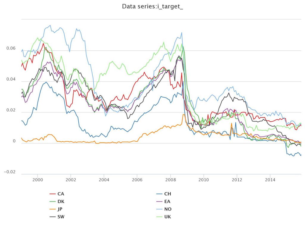
Figure 1: 3-months yields on Eurocurrency deposits
Second, we now have more indicators for risk aversion for extended period of time. This potentially allows us to distinguish between competing explanations for the failure of the unbiasedness hypothesis. Specifically, we can examine whether the inclusion of these risk proxies alters the Fama puzzle.
The New Puzzle
We obtain the following findings. First, Fama’s (1984) finding that interest rate differentials point in the wrong direction for subsequent ex-post changes in exchange rates is by and large replicated in regressions for the full sample, ranging from 1999 to February 2016. However, the results change if the sample is truncated to apply to only the most recent decade, the period for which interest rates are essentially at zero. For that period, interest differentials correctly signal the right direction of subsequent exchange rate changes, but with a magnitude that is altogether not reconcilable with the arbitrage interpretation of UIP. In other words, we obtain positive coefficients at exactly a time of high risk when it would seem less likely that UIP would hold. This finding is illustrated for eight exchange rates (against the USD) in Figure 2, at the three month horizon.
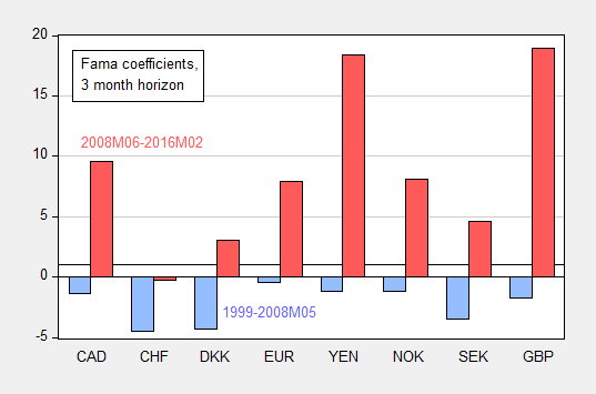
Figure 2: OLS regression coefficient of ex post depreciation on interest differential, at three month horizon, for 1999-2008M05 (blue bar), and 2008M06-2016M02 (red bar).
For greater insight into how the correlations look before and after the global financial crisis, Figure 3 presents a scatterplot for the UK-US relationship, again at the three month horizon in Figure 3.

Figure 3: 3-month ex post depreciation of USD against British Pound vs corresponding 3-month US-UK yield differential: Pre-crisis versus post-crisis
Is It (Mostly) Risk? Or Expectations?
We also find that the inclusion of a proxy variable for risk, namely the VIX, results in Fama regression coefficients that are only slightly more in line with anticipated values of unity. This finding suggests that changes in the elevation of risk as measured by the VIX do not explain the forward rate bias, at least not in a direct linear fashion.
The use of expectations data provides the following insights. First, interest differentials and anticipated exchange rate changes are positively correlated, consistent with the proposition that investors tend to equalize at least partially expected returns expressed in common currency terms (see also Chinn and Frankel (2016) for results 1986-2009). Second, in cases where the Fama coefficient switches sign from negative to positive from pre- to post-crisis (euro, yen against USD), the result arises because the correlation of expectations errors (defined as expected minus actual) and interest differentials changes substantially between pre- and post-crisis periods.
plim(β’) = 1 – [A] – [B] – [C]
Where β’ is OLS regression coefficient from the Fama regression:
s+1 – s = α’ + β'(i-i*) + error
[A] ≡ cov(covered interest diff.,i-i*)/var(i-i*)
[B] ≡ cov(risk premium, i-i*)/var(i-i*)
[C] ≡ cov(forecast error, i-i*)/var(i-i*)
covered int. diff. = – [(f – s) – (i-i*)]
risk premium = f – ε(s+1)
forecast error = ε(s+1) – s
ε(s+1) is subjective market expectations of the future spot exchange rate (proxied using Consensus Forecasts survey data).
When it doesn’t switch (Swiss franc), the expectations-interest component does not switch sign. This pattern is shown in Figures 4-6, for the euro, yen, and Swiss franc against the USD, at the three month horizon.
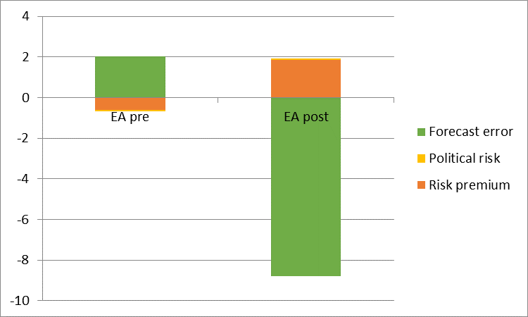
Figure 4: Decomposition of deviation of coefficients from unity for Euro
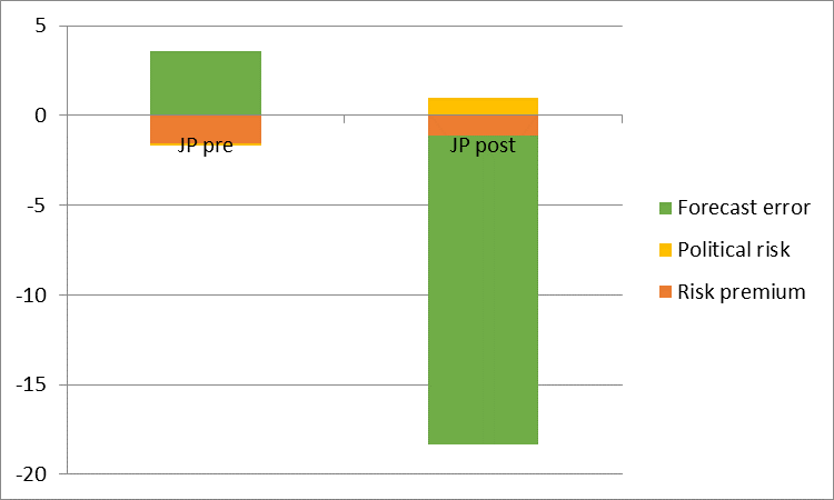
Figure 5: Decomposition of deviation of coefficients from unity for Yen
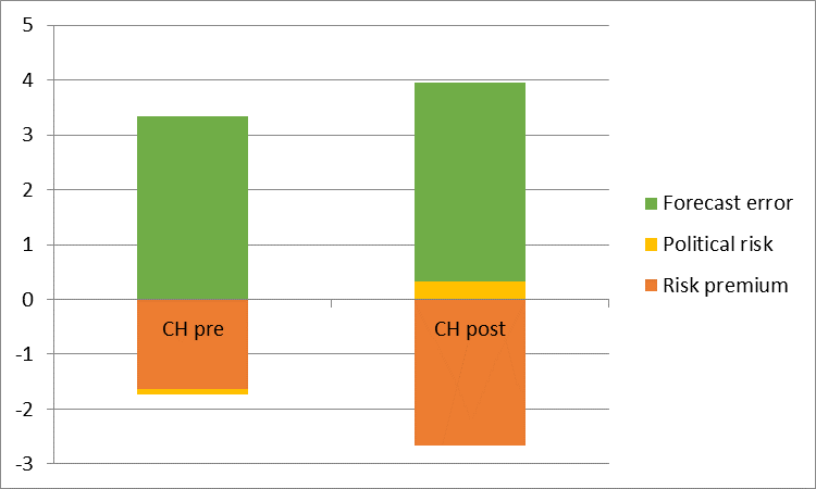
Figure 6: Decomposition of deviation of coefficients from unity for Swiss franc
Concluding Thoughts
Exchange risk comovement with the interest differential does not appear to be the primary reason why the Fama coefficient has been so large in recent years (although the altered behavior of exchange risk does play a role). Rather, how expectations errors comove with the interest differential appears of central importance.
Dear Menzie,
This is going to be a stupid comment, but since no one else will mention this, I will risk being an idiot. If the expectations errors are small, so they might be within confidence intervals of some sort of forecasting equation, might the results be different than if expectation errors are large? Yes, it will be dependent on whatever forecasting equation you use, but some sort of a generic one might allow a question like this to be answered.
Julian
Menzie – thanks for this insightful update on an issue that not only has a long history but is also timely in a lot of different ways.