In a new paper, Ryan LeCloux (Legislative Reference Bureau) and I discuss the challenges to assessing the economic outlook at the state level. We examine the various indicators available to track macroeconomic indicators at the higher than annual frequency. We find that quarterly GDP at the state level is correlated with different macroeconomic indicators for different states. Hence, tracking the economic activity of each state accurately might require focus on different variables.

The Coherence between GDP and Other Macro Aggregates

Contrary to some speculation, the Philadelphia Fed’s coincident index is a fairly effective indicator of GDP. In 72% of the cases, the correlation of log first differences is positive and statistically significantly so. Next consider a sensitivity coefficient obtained from the following specification:

Δy_t = α + βΔx_t + ε_t

Where y ≡ ln(Y), so Δy is the essentially the growth rate on a quarterly basis of real GDP, while Δx is the growth rate of either real income, nonfarm payroll employment, civilian employment or the coincident index. The results of this regression are shown in Table 2 from the paper.

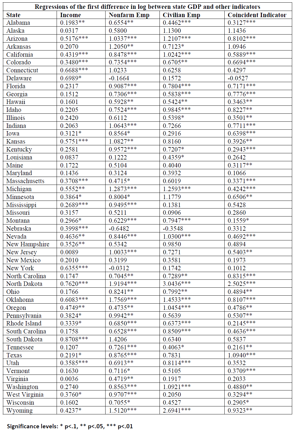
Table 2 from Chinn-LeCloux (2018).

The sensitivity of GDP growth to coincident index growth (the estimated β coefficient) varies from 0.29 (Wisconsin) to 2.5 (North Dakota), in the cases where the coefficient estimates are significantly different from zero. The latter is somewhat of an outlier; the next highest sensitivities are 1.095 (Akransas) and 1.094 (Texas). A geographic depiction of the sensitivities is shown in Figure 9 from the paper.

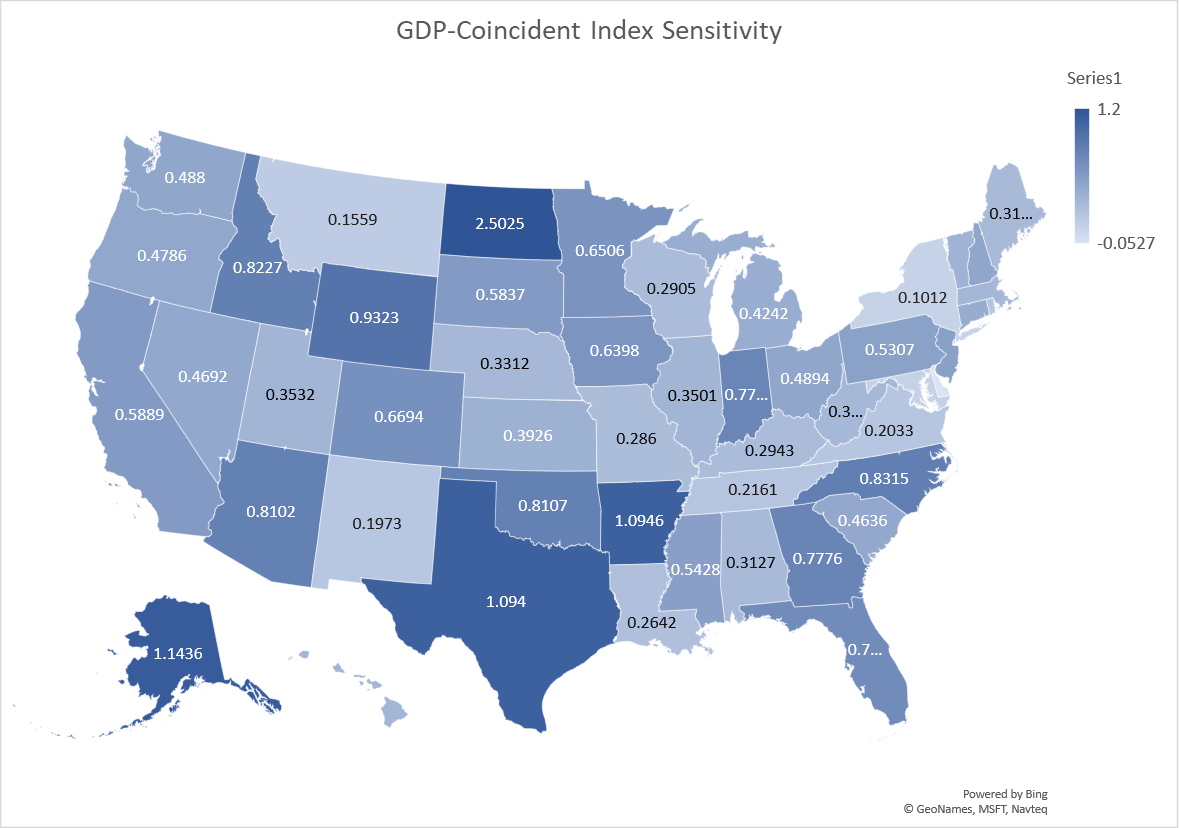
Figure 9 from Chinn-LeCloux (2018): Sensitivity of GDP growth to Coincident Indicator growth, quarter-on-quarter.

The following figure is a histogram of the estimated β’s.

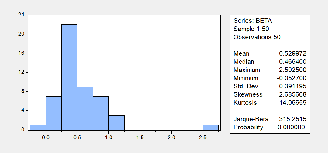
Figure 1: Histogram of estimated β’s.

At various junctures, certain observers have criticized the use of the Philadelphia Fed coincident indicators (e.g., [1], [2], [3]; Ironman asserted cross-state comparison of these indices is an example of “junk science”), and advocating the use of civilian employment, to track economic activity in Kansas, or Wisconsin. In the paper, we spend some time discussing why the civilian employment series from the household survey is a particularly difficult series to use in real time tracking of state level economies.

Assuming GDP is the best proxy measure for economic activity, it looks like the coincident indicator, income and nonfarm payroll employment are good proxies; civilian employment is not. For Kansas, the coincident index is highly significantly correlated with GDP, with a sensitivity of 0.39. For Wisconsin, nonfarm payroll employment and the coincident indicators are significantly correlated. The sensitivity of GDP growth to coincident growth is 0.29.

Some states do not exhibit any correlation of GDP with any of the standard measures: Alaska, Maryland, Missouri, and New Mexico. Interestingly, for New York state GDP only correlates only with personal income.

Using Quarterly GDP Data to Compare Performance against a Counterfactual

In one section of the paper, we use the quarterly GDP series for Kansas to assess whether the 2012 tax cut legislation, fully implemented in calendar year 2014, had the desired effect. At the time, Governor Brownback asserted that the tax program would act like a “shot of adrenaline”. The outstanding question then is whether output rose as a consequence of this measure.

As we note in the paper, this is a difficult question to answer completely, as it would require a fully fleshed out model, with explicit stances taken on causality, and the channels whereby which the tax measure affected economic behavior. With minimal data available at high frequency and in near reeal time, what can one do?

A reasonable approach is to see if output differed from what it otherwise would have been in the case of no tax cut. That requires the construction of a counterfactual, taking a stand on what is kept constant and what is not. We construct a counterfactual GDP series by using data from 2005-2013 period (2005 is the beginning of the quarterly state GDP series, 2013 is just before the tax plan is fully implemented.)

The counterfactual is created using an estimated error correction model, where c is a real commodity price index for Kansas.

Δy_t^KS = 0.478 – 0.190 y_t-1^KS + 0.182 y_t-1^US + 0.945Δ y_t^US + 0.123Δc_t-1 + u_t

Adj-R² = 0.42, SER = 0.0124, N = 35, Sample 2005Q2-2013Q4. DW = 2.04, Breusch-Godfrey Serial Correlation LM Test = 1.19 [p-value = 0.32]. Bold face denotes statistical significance at 10% msl, using HAC robust standard errors. The Box-Ljung q-statistics for up to 8 lags does not reject the null of no serial correlation.

This model, when simulated dynamically out of sample, using realized values of US GDP and the real commodity price (what is called an ex post historical simulation) yields the following conclusions:

We find that actual Kansas GDP is at times far below predicted (5.9 billion Ch.2009$ SAAR, or 4.2%, as of 2017Q3). In other words, given the evolution of US GDP and commodity prices, and the historical correlations that held until 2013Q4, economic output was below expected. However, given the imprecision of the estimates, the shortfall is not statistically significant, even at the 40% level.

This result is shown in Figure 12 from the paper.

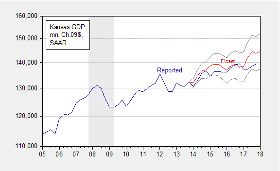
Figure 12 from Chinn-LeCloux (2018): Kansas GDP as reported (blue), and forecast (red), and 60% prediction interval (gray lines), all in millions Ch.2009$, SAAR. NBER defined recession dates shaded gray.

In another assessment, using a longer sample of data on coincident indices, which affords more precise estimates, I’ve found the gap to be statistically significant. (By the way, one analyst appealed to drought as an explanation for underformance, by subtracting out agriculture; but in that case, they did the subtraction of real terms incorrectly, invalidating the analysis.)

Conclusion

With the advent of quarterly GDP series, analysts are better armed to analyze business cycle developments in state level economies than they were before. Nonetheless, other indicators — employment, income and the Philadelphia Fed’s coincident indicators — will continue to be of use, perhaps even more useful in some cases than others.

The paper is here. Constructive comments welcome.