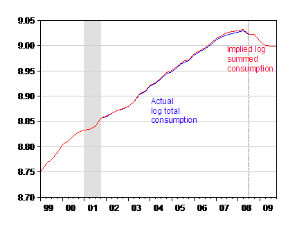
Suppose by 2009Q4, GDP is 0.13% below 2008Q3 levels, real equity wealth is 35.2% below end-June levels, and real nonequity wealth is 6% below end-June levels. Further assume that the real Fed Funds rate remains at 2008Q3 levels (-2.45%). Then, the conditional estimate of 2009Q4 consumption will be 2.16% below 2008Q3 levels. This implies a 3% y/y decline in consumption by 09Q3; the only comparable instance of such a decline is 1951Q3, when consumption declined y/y by 2.3% (all percent calculations in log terms).
Figure 1 depicts the path of consumption under these assumptions, and using error correction models for durables and nondurables consumption, and a AR in first differences for services consumption.

Figure 1: Log real total consumption (blue) and log sum of forecasted consumption components (red), in Ch.2000$, SAAR. NBER defined recession dates shaded gray. Dashed line indicates beginning of forecast period. Source: BEA, NIPA release of 30 October, NBER, and author’s calculations.
Note that I have taken the expedient of adding together the chained spending series (in Chained 2000$) even though chained series do not obey additivity constraints (see [1]). This shortcut does not appear to do too much violence to the data, as illustrated by the small gap between the blue and red lines.
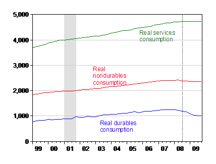
Here are the disaggregated real consumption levels, in Ch.2000$.

Figure 2: Real durables consumption (dark blue) nondurables consumption (pink) and services consumption (dark green), in Ch.2000$, SAAR. NBER defined recession dates shaded gray. Dashed line indicates beginning of forecast period. Source: BEA, NIPA release of 30 October, NBER, and author’s calculations.
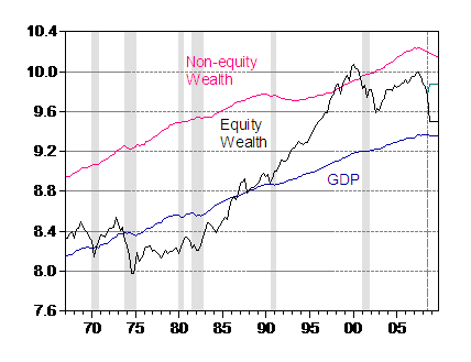
The assumptions I’ve made for the explanatory variables are shown below.

Figure 3: Log real GDP (dark blue), log real non-equity wealth (pink), and log real equity wealth (black), and alternate log real equity wealth (teal), in Ch.2000$, SAAR. NBER defined recession dates shaded gray. Dashed line indicates beginning of forecast period. Wealth variables deflated by consumption expenditure deflator. Non-equity wealth and equity wealth calculated using flow of funds data as in Carroll, Otsuka, Slacalek (2006). Source: BEA, NIPA release of 30 October, Federal Reserve Board Flow of Funds, NBER, and author’s calculations.
The trajectories displayed above assume: (i) equity wealth move with S&P500, and hold constant at Nov. 11 levels in real terms from 2008Q3 onward; (ii) real nonequity wealth declines at 1% per quarter (in log terms) from 2008Q2 onward. This compares with a 2.3% per annum decline for the two years following the 1990-91 recession. The GDP forecast is from the October 17, 2008 Deutsche Bank forecast (shown here).
The equations used are estimated over the 1969Q1-08Q3 period. They are:
Durables
Δc_durt = -1.49 – 0.18 (c_durt-1) + 0.14 (yt-1) – 0.33 r t-1 + 0.04 we t-1 + 0.10 wn t-1 + three lags of first differences + u t
Adj.R2 = 0.25, N=159, SER = 0.027, DW = 2.05; bold face denotes significant at 10% msl. we is equity wealth, wn is non-equity wealth.
- Long run income elasticity: 0.78.
- Long run interest semi-elasticity: -1.81.
- Long run equity wealth elasticity: 0.23.
Nondurables
Δc_ndur t = 0.006 – 0.07 (c_ndur t-1) + 0.03 (y t-1) – 0.05 r t-1 + 0.006 we t-1 + 0.10 wn t-1 + three lags of first differences + u t
Adj.R2 = 0.20, N=159, SER = 0.006, DW = 1.86
- Long run income elasticity: 0.43 (significant at 20% levels).
- Long run interest semi-elasticity: -0.81.
- Long run equity wealth elasticity: 0.09 (significant at 20% levels).
- Long run nonequity wealth elasticity: 0.28 (significant at 20% levels).
Services
Δc_svcs t = 0.028 – 0.003 (c_svcs t-1) + 0.20 ( Δ c_svcs t-1) + 0.07 Δ(y t-1) – 0.14 ( Δ r t-1) – 0.09 ( Δ r t-3) + 0.036 ( Δ networth t-1) + 0.030 ( Δ networth t-3) + other nonsignificant lags of first differences + u t
Adj.R2 = 0.28, N=159, SER = 0.0036, DW = 2.06
- Short run income elasticity: 0.35.
- Short run interest semi-elasticity: 1.18.
- Short run net worth elasticity: 0.44.
This projection would place the log ratio of consumption to GDP in 2009Q4 at the same levels that it was in 2000.
Time for (lots of) caveats:
- The estimated coefficients are sensitive to the selection of specifications. I have searched for error correction model (ECM) specifications with 3 lags of first differences and a common set of determinants (income, household equity and household non-equity wealth, real interest rate). Three lags of first differences are consistent with 4 lags of the VAR representation of the VECM. I checked to see if the residuals then exhibited serial correlation. (Note Carroll et al. (2001) argues that the ECM approach is not appropriate.).
- I did not adopt a formal general-to-specific modeling methodology. Variables with non-significant coefficients were retained. Additional searching would surely lead to other plausible specifications.
- The coefficient estimates are sensitive to specification. However, I think the long run elasticities reported above are not implausible (although I am willing to be corrected). For instance, Alexander and Slok (2001) report for total consumption a long run equity wealth elasticity of 0.08, and 0.04 for housing wealth. While the corresponding long run elasticities are higher in the above specifications, it’s important to recall that in particular durables is a small share of consumption total (10%), while nondurables is about 30%. Services, with no estimated long elasticity, constitutes the remaining 60% of consumption.
- I could not obtain an ECM specification for services consumption that incorporates long run effects income, net worth, and real interest rates.
- I did not include the relative price of durables in the durables consumption equation. This is true even though the variable shows up as significant, and exhibits a definite trend ([1]), because incorporating it into the projection would require taking a stand on the future trajectory of yet another variable.
- The projection are sensitive to the assumptions regarding the path of the exogenous (for purposes of the simulation) variables.
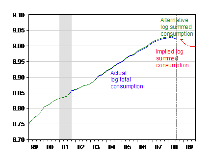
Returning to this last point, consider what happens if I assume the household equity wealth returns to 2008Q1 levels (as shown in the teal line in Figure 3).

Figure 4: Log real total consumption (blue), log sum of forecasted consumption components under baseline (red), and log sum of forecasted consumption components when real household equity wealth rebounds to 2008Q1 levels (green), in Ch.2000$, SAAR. NBER defined recession dates shaded gray. Dashed line indicates beginning of forecast period. Source: BEA, NIPA release of 30 October, NBER, and author’s calculations.
The consumption decline (as shown in the green line) is much less marked.
This leads me to my key take-away. Don’t think of the above as so much a forecast as a projection conditional upon a number of assumptions, where I’m sure some readers will take them as either too optimistic or too pessimistic. From my perspective, the main point is one’s projection of consumption’s path will depend in large part on the path for equity (and non-equity) household wealth.
[Update 11/19 7:25pm Pacific: more on consumption from Morgan Stanley: “Perfect Consumer Storm to Last Until Mid-2009
“.]
Technorati Tags: recession, consumption,
stock market, and credit crunch.
If the consumption model is sensitive to changes in household wealth, that seems right. Maybe it should also be sensitive to major changes from long term averages of unemployment. In the multiple regression world, equity wealth and unemployment may be (negatively) correlated. In the real world, rapid changes in unemployment off the long term average causes changes in consumption behavior in a different, and larger, group of people than those folks who are directly influenced by their monthly mutual fund statement. FWIW.
Mike Laird: I agree, there are lots of additional candidatevariables. One that’s missing is a proxy measure for uncertainty, which would make sense in a buffer stock model of consumption. In principle GDP proxies for unemployment (I tried labor income as well in results not reported), and wealth for life-cycle effects.