Today we are fortunate to have a guest contribution written by Roberto Duncan, assistant professor of economics at Ohio University.

---

In spite of the current account reversals observed in advanced countries, global imbalances are still a matter of concern (IMF, 2014). Probably, the US current account is the most important component of such worldwide imbalances. The size of the US external deficit has been an issue of analysis for many years. Research on this specific topic has used, at least, two approaches. On the one hand, some researchers contend that thresholds in the dynamics of the current accounts exist. The simplest threshold model can be understood as one where a threshold value is used to identify ranges of values where the behavior predicted by the model varies in some relevant way. For example, Clarida, et al. (2005) find two thresholds in the US current-account-to-GDP ratio. According to that, if the current account surplus is above 2.2% or below -2.2% of GDP, we should expect a reversal toward its long-run mean. Usually, these papers employ only the information contained in the time series of the current account itself (a univariate approach). On the other hand, a number of works based on dynamic stochastic general equilibrium (DSGE) models suggest that the US current account is driven by shocks of fiscal balance, productivity level, productivity volatility, or oil prices.¹

Even though a nonlinear univariate model might be useful –for example, for forecasting purposes– its nature leaves aside the fundamentals behind the current account dynamics. The DSGE literature, in turn, usually focuses on linear(ized) relationships and emphasizes one or two factors –partly due to the curse of dimensionality. In the paper titled “A Threshold Model of the US Current Account”, I aim to bridge the gap between these two branches in a multivariate nonlinear framework that can offer more tractability. I address several questions: What are the main drivers of the US current account? Is the behavior of the current account the same during deficits and surpluses or does the size of the external imbalance matter as some analysts suggest? Is there a threshold relationship between the current account and its drivers?

To answer these questions, I estimate a threshold model with multiple regressors to explain the behavior of the US current account during the period between 1973.I and 2012.I, and test for the presence of regimes in its dynamics. As threshold candidates, I try a set of variables suggested by commentators and previous empirical works: the (lagged) level and the size of the current account-to-GDP ratio, the (lagged) level and the size of the fiscal-balance-to-GDP ratio, and time. In the latter case, I actually test for the presence of an unknown time break in the relationship between the regressors and the dependent variable. As regressors, I evaluate a similar set to the one proposed in the DSGE literature mentioned above. In addition, I include the real interest rate and the real exchange rate.²
To deal with the potential endogeneity of the regressors, I use the IV estimator of a threshold model developed by Caner and Hansen (2004).

Main findings

First, in contrast to the univariate threshold models, time is the most important threshold variable. I find a robust time break –not previously documented in the literature– in the relationship between the current account and its main drivers in the third quarter of 1997. Our estimates stubbornly point to 1997.III as the time break even if I use a larger sample such as 1957.I-2012.I.

The time break found in 1997.III coincides with two events: the onset of the Asian financial crisis and the Taxpayer Relief Act of 1997. The former implied a recomposition of portfolios among international investors, including central banks, and the decision of sharp devaluations, the imposition of capital controls, and reserves buildup by monetary authorities. In addition, the Asian financial crisis is viewed as the onset of a sequence of international crises among emerging market economies. Other economies that faced similar crises were Russia (1998), Brazil (1998), Argentina (1999-2002), and Turkey (2001). All of them involved sharp devaluations, modification of the exchange rate regime, and the rise of foreign exchange reserves as a hedge against potential speculative attacks or another financial crisis. While the change in exchange rate policies to limit currency appreciations has led to some to talk about a revived Bretton Woods system (Dooley et al., 2003), the war chests of foreign reserves have, at least in part, led to an increasing purchase of US treasury bonds, which is usually linked to the so- called global saving glut hypothesis (Bernanke, 2005). The second factor that might have contributed to the structural change originated domestically. The Taxpayer Relief Act of 1997, enacted on August 5th, reduced several federal taxes, provided some tax exemptions, and extended tax credits. According to estimates posted by the NBER, the average marginal tax on long-term gains was reduced by almost 7%, from 25.6% to 18.7% in 1997, the largest cut since 1960.

Second, as opposed to what other authors contend, I did not find evidence on the importance of the size or the sign of the current account as threshold variables. The time line always dominates any potential threshold variable previously used or proposed by the empirical literature in terms of model fit. The other candidate variables not only fail to provide an adequate fit compared to the time line, but also they are highly sensitive to the sample, and did not provide either precise threshold or coefficient estimates, or statistics that could support a valid model in each regime.

Third, the most significant determinants of the US current account are total factor productivity, the real exchange rate, the fiscal surplus, and the volatility of productivity in both regimes (before and after 1997.III). As the paper shows, the most statistically significant shifts are related to the productivity level, the real exchange rate, and the real interest rate. In particular, productivity shocks became more important after 1997.

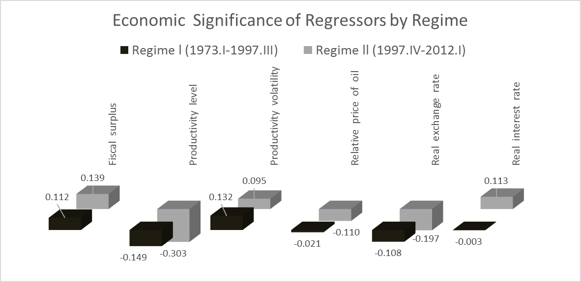
The figure above displays the economic significance of each regressor. That is, the coefficient estimate multiplied by the standard deviation of the corresponding regressor. For example, one-standard-deviation shock in productivity lowers the current account in approximately 0.15 points of long-run GDP in the pre-1997 regime, whereas the respective reduction is 0.3 points of long-run GDP in the post-1997 regime.

Fourth, the relative price of oil and the real interest rate become statistically significant and more economically relevant after 1997, although shocks to these relative prices do not contribute significantly to fluctuations in the current account surplus, at least as much as other regressors of the model. For example, a one-standard-deviation shock in the interest rate would be associated with a rise in the current account of 0.11% of long-run GDP. From an economic viewpoint, the saving glut effect through the interest rate is relatively less important. Similarly, a one-standard-deviation shock in oil prices above its trend would be related to a current account decline of 0.11 percentage points of long-run GDP.

Why did productivity shocks become more important after 1997?

We mentioned that the time break coincides with the onset of the Asian financial crisis. One possibility is that international investors moved their funds from East Asia and, perhaps, other emerging market economies, to the US and invested in more capital-intensive sectors such as the information industry.³ The best example of this investment shift could have been the dot-com bubble observed between 1997 and 2000. The capital intensification of the economy could have made productivity shocks a more important driver of investment and, as a result, the current account. To a lesser degree, another possibility is that the Taxpayer Relief Act of 1997 raised the sensitivity of domestic absorption and, consequently, the sensitivity of the current account to productivity shocks.⁴

To summarize, we find that time is the best threshold variable in the dynamics of the US current account. In particular, one regime exists before and another one exists after the third quarter of 1997, a period that coincides with the onset of the Asian financial crisis and the Taxpayer Relief Act of 1997. Productivity has become a more important driver of the US current account since then. Further research is needed to verify the reason behind this fact. An important implication for practitioners, who seek to improve the fit of their models that attempt to explain the current account deficit, is the need of taking into account the 1997 structural break and modeling it in a DSGE framework. Such task could be one of the next steps in the research agenda on global imbalances.

References

Acemoglu, D., Guerrieri, V., 2006. Capital deepening and non-balanced economic growth. NBER Working Paper 12475.

Bernanke, B., 2005. The Global Saving Glut and the U.S. Current Account Deficit. Remarks at the Sandridge Lecture, Virginia Association of Economists, Richmond, Virginia. The Federal Reserve Board.

Bodenstein, M., Erceg, C.J., Guerrieri, L., 2011. Oil shocks and external adjustment. J. Int Econ. 83, 168-184.

Bussiere, M., Fratzscher, M., Muller, G., 2010. Productivity shocks, budget deficits and the current account. J. Int. Money Financ. 29, 1562-1579.

Caner, M., Hansen, B., 2004. Instrumental Variable Estimator of a Threshold Model. Economet. Theor. 20, 813-43.

Chinn, M., Prasad, E., 2003. Medium Term Determinants of Current Accounts in Industrial and Developing Countries: An Empirical Exploration. J. Int Econ. 59(1), 47-76.

Clarida, R., Goretti, M., Taylor, M., 2005. Are There Thresholds of Current Account Adjustments? NBER conference G7 Current Account Imbalances: Sustainability and Adjustment.

Dooley, M., Folkerts-Landau, D., Garber, P., 2003. An Essay on the Revived Bretton Woods System, NBER Working Paper No. 9971.

Duncan, R., 2015. A Threshold Model of the US Current Account, forthcoming in Economic Modelling.

Fogli, A., Perri, F., 2006. The Great Moderation and the U.S. External Imbalance. Monetary and Economic Studies (Special Edition). 209-234.
International Monetary Fund, 2014. World Economic Outlook, Legacies, Clouds, Uncertainties (October).

---

^{1. See Bussiere, et al. (2010), Fogli and Perri (2006), and Bodenstein, et al. (2011), respectively. Another branch of the empirical literature centers its attention to medium-term fluctuations of the current account using cross-country samples (e.g., Chinn and Prasad, 2003) and overlaps with the DGSE branch. The inclusion of demographic regressors, for example, is more appropriate in cross-country regressions rather than time-series models due to their low variability over time.}

^{2. A reduction in this index indicates real currency depreciation.}

^{3. According to Acemoglu and Guerreri (2006), the information sector in the US has a capital share of 0.53 (the average capital intensity is around 0.4).}

^{4. Consider, for simplicity, an economy in which a productivity shock raises dividends and, therefore, generates capital gains. If capital gains are taxed at the rate t, then consumption would increase by a proportion that depends on 1-t. If such tax rate is reduced, the sensitivity of consumption to productivity shocks would increase.}

---

This post written by Roberto Duncan.