That’s the title of a new paper, coauthored with Yin-Wong Cheung, Antonio Garcia Pascual, and Yi Zhang.
In an era characterized by increasingly integrated national economies, the exchange rate remains the key relative price in open economies (see surveys, Engel (2014), Rossi (2013)). As such, a great deal of attention has been lavished upon predicting the behavior of this variable. Unfortunately, it is unclear how much success there has been on this front. Beginning with the work of Meese and Rogoff (1983), many economists have evaluated exchange rate models using a horse race approach: see which model performs the best in predicting the actual level of the exchange rate when it’s assumed the determinants are assumed to be known. Earlier studies focused on a fairly narrow set of models, including ones where interest rate differentials, monetary factors, and foreign debt, mattered. In more recent studies (Cheung, Chinn, and Garcia Pascual, 2005) this set of models were augmented by those including a role for price levels, for productivity growth, and a composite specification incorporating several different channels whereby which both debt, productivity and interest rates matter (i.e., behavioral equilibrium exchange rate, BEER, model).
In this paper, we examine the British pound, Canadian dollar, the euro, Japanese yen, and Swiss franc, all against the US dollar. The euro is newly included relative to our 2005 paper, supplanting the Deutsche mark.
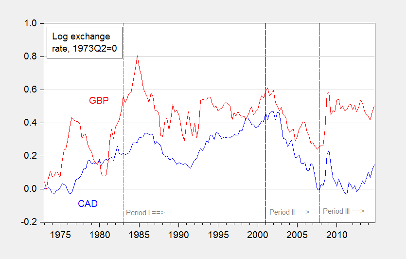
Figure 1: Exchange rates for Canadian dollar and British pound, end of month.
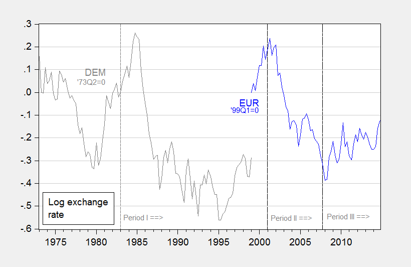
Figure 2: Exchange rates for Deutsche mark and euro, end of month.
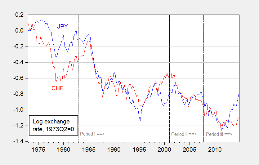
Figure 3: Exchange rates for Japanese yen and Swiss franc, end of month.
The set of models is further expanded to include the factors that central banks are believed to pay attention to – so called “Taylor rule fundamentals” (e.g., Molodtsova and Papell, 2009) such as the degree of slack in the economy, and the inflation rate –, the difference between short and long term interest rates – sometimes called the slope of the yield curve (e.g., Chen and Tsang, 2013). In this study, the analysis also addresses the special factors that have characterized the world economy over the last decade, including the fact that it is difficult to set interest rates much below zero (i.e., the advent of the zero lower bound), and the rise of importance in risk and liquidity in global financial markets. We account for the former by use of what are called “shadow interest rates”, i.e., the short term interest rate consistent with longer term interest rates. We account for the latter by augmenting standard models based on monetary fundamentals with measures of risk, namely the VIX and the TED spread.
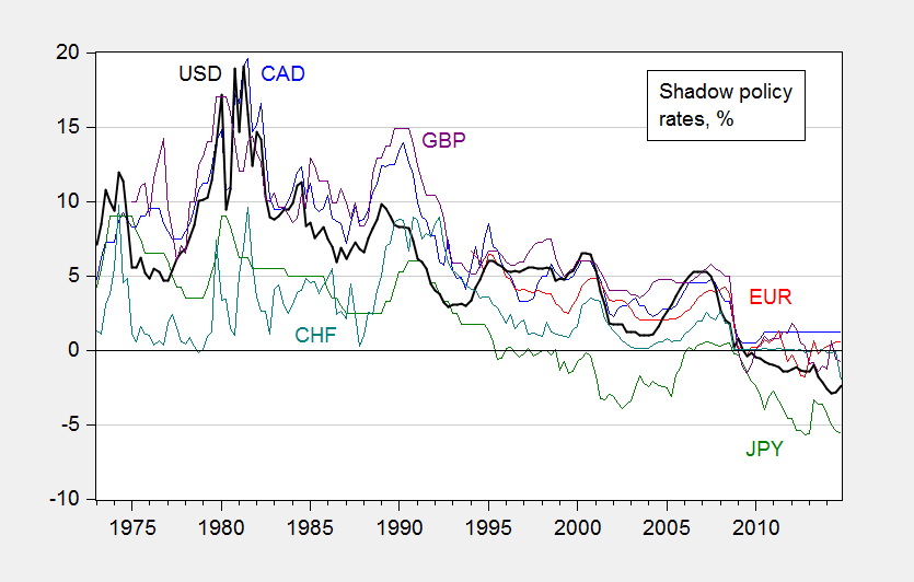
Figure 4: Overnight interest rates and shadow rates.
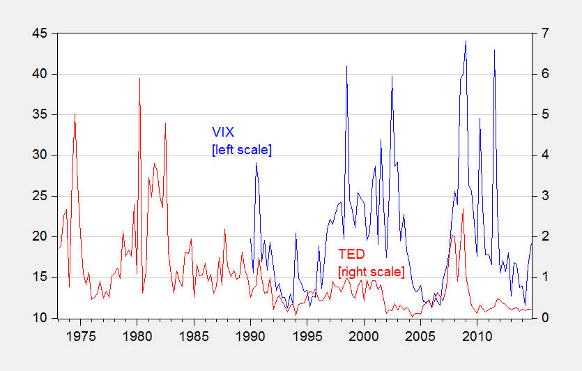
Figure 5: VIX (left scale) and TED spread (right scale).
The performance of each of these models is compared against the “no change”, or random walk, benchmark, and over different time horizons (1 quarter, 1 year, 5 years), using differing metrics. The first metric is whether the variability of the predictions around the actual values is greater than or less than that obtained by a “no-change prediction”. This is a comparison of the mean squared error of a model against a random walk model. The second metric is a direction of change comparison – does the predicted change in the value of the exchange rate match the actual change. The third metric is a “consistency” test, proposed by Cheung and Chinn (1998). This test requires that the predicted value and the actual exchange rate share the same trend.
Because it’s not known whether the form of the relationships, we use two specifications. The first is to assume that the level of the exchange rate is related to the level of explanatory variables, over the long term. In this approach, if the level of the exchange rate is below the level predicted in the long run by the explanatory variables, then the exchange rate will be predicted to rise. The second is to assume the growth rate of the exchange rate as depending on the growth rate of the explanatory variables.
Finally, in order to ensure that our findings are not being driven by our selection of time periods to examine the performance of the models, we conduct the comparisons over three different periods, as shown in Figures 1-3: (i) the period after the US disinflation (starting in 1983), (ii) the period after the dot.com boom (starting in 2008), and (iii) the period starting with the beginning of the Great Recession (the end of 2007).
In summary, no model consistently outperforms a no-change – or random walk – prediction, by a mean squared error measure, although the model that predicts a relationship between differences in price levels and the exchange rate – “purchasing power parity” — does fairly well. Overarching these results, specifications incorporating long run relationships in levels tend to outperform specifications involving growth rates, particularly along the mean squared error dimension.
The models that have become popular in last fifteen years or so might not be much better than the older ones. Overall, the results do not point to any given model/specification combination as being very successful, on either the mean squared error or consistency criteria. On the other hand, many models seem to do well, particularly using the direction of change criterion.
Of the economic models, purchasing power parity and interest rate parity do fairly well, perhaps due to the parsimoniousness of the specifications (interest rate parity requires no parameter estimation). In the most recent period, accounting for risk and liquidity tends to improve the fit of the workhorse sticky price monetary model, even if the predictive power is still unimpressive. But in general the more recent models do not consistently outperform older ones, even when assessed on the recent, post-crisis period.
The euro/dollar exchange rate appears particularly difficult to predict, using the models examined in this study. This outcome is likely attributable to the short span of data available for estimating precisely the empirical relationships.
References
Cheung, Yin-Wong, Menzie Chinn, and Antonio Garcia Pascual, 2005, “Empirical Exchange Rate Models of the Nineties: Are Any Fit to Survive?” Journal of International Money and Finance 24 (November): 1150-1175. Also NBER Working Paper no. 9393 (December 2002).
off topic :
Hi Menzie, this is something interesting for you:
Wisconsin governor Scott Walker and his cash cows:
https://www.theguardian.com/us-news/2016/sep/14/corporate-cash-john-doe-files-scott-walker-wisconsin
Hope you are able to get a copy of the file, before it’s too late.
Enjoy !