Today, we are pleased to present a guest contribution written Hiro Ito (Portland State University). This web post was posted in RIETI’s columns series.
There is no doubt that the U.S. dollar is the most dominant international currency in many aspects of international finance. It has the largest market share in international trade settlement and invoicing, investment and financial settlements, and foreign exchange market transactions. Moreover, the world’s central banks hold more than 60% of their foreign exchange reserves in US dollars. According to Ito and Kawai (2024), 35-38% of global GDP uses the dollar as an anchor currency. To date, no credible currency has emerged as a competitor to the U.S. dollar.
The dollar’s dominance in the international monetary system has created a world in which shocks to the dollar’s issuer, the United States, spill over to other countries. Spillovers from the U.S. affect global asset markets, bank lending, and economic fluctuations. In such a system, the non-U.S. world watches U.S. monetary policy decisions and other economic and financial news as if it were its own policy and economic data.
Despite the obvious dominance of the U.S. dollar, measuring the size of a currency’s dominance zone is a rather tedious task. The dominant method of estimation is the subject of academic controversy.
A recent paper by Ito and Kawai (2024) developed a new method for estimating the size of major currency areas: the US dollar (USD), the euro (EUR), the Japanese yen (JPY), the British pound (GBP), and the Chinese yuan (RMB). This paper employs a simple econometric approach, first popularized by Frankel-Wei (1994) and further developed by Kawai-Pontines (2016), to estimate the size of major currency areas.
Specifically, the depreciation rate of a country’s currency X against a numerical currency (e.g., the New Zealand dollar) is regressed on the depreciation rates of the five major currencies. This estimation yields estimated coefficients for each of the major currencies. By running this estimation in a rolling window, the time-variant share of each major currency is obtained. If a currency is pegged to the U.S. dollar (e.g., the Hong Kong dollar), the estimated coefficient of the exchange rate against the dollar is 1 and the estimated coefficients for the other major currencies are zeros. If, for example, the estimated coefficients are found to be (USD, EUR, GBP, JPY, RMB) = (0.40, 0.40, 0.05, 0.05, 0.10), the estimated weights are 40% for the USD, 40% for the EUR, 5% each for the GBP and JPY, 10% for the RMB, etc.
This approach has two inherent drawbacks. First, if some of the major currencies are correlated with each other, the estimated weights are not statistically accurate. The Chinese yuan was explicitly or implicitly pegged until recently, which could bias the estimates. Second, many researchers use the estimated coefficients as weights for major currencies in a currency basket, but the statistical significance of the estimated results is usually not factored in. Therefore, there is a risk that the size of the currency zone is overestimated. In particular, it has been argued that the size of the yuan zone has expanded in recent years. However, there do not appear to be any papers that discuss whether the estimation coefficients needed to estimate the size of that currency zone are statistically significant. In other words, the size of the RMB (or other) zone is likely overestimated. In other words, the RMB zone could be much smaller than many have been estimated.
Ito and Kawai (forthcoming RIETI working paper) carefully address these two issues. For the issue of potentially high correlations among major currencies, they implement the Kawai and Pontines (2016) method to reduce bias arising from potentially high correlations among major currencies.
As for the second issue, the paper considers the degree of ERS, defined by the Root Mean Squared Error (RMSE) of the estimation model. A higher level of the RMSE means a lower level of goodness of fit, therefore, a lower level of ERS (a more flexible exchange rate regime). The estimated currency weights are multiplied with ERS so that the weights would be higher if the level of ERS is higher (i.e., a lower RMSE, leaning toward more exchange rate stability), whereas a higher RMSE means lower ERS (i.e., more flexible exchange rate regime). With this modification, overestimating the size of a particular major currency zone, such as the RMB zone, can be avoided. In other words, the Ito and Kawai (2024) approach identifies both to what extent a country belongs to each of the major currency zones, and how statistically significantly that is. Hence, this approach can avoid overestimating the size of currency zones, and inevitably shows more flexible exchange rate regimes. By more delicately specifying the exchange rate regime, not only in terms of which major currency the home currency is stabilized to, but also in terms of how “tight” (or “loose”) it should be considered statistically, this approach can present a picture that is more consistent with the current state of the international monetary system.
Figure 1 provides snapshots on the evolution of exchange rate regimes over the past 50 years by focusing on anchor currencies and the degrees of exchange rate stability (or flexibility) for individual economies. Each economy in the world map is colored based on the anchor currency with the statistically significant, highest-estimated weight among the major currencies. For example, in the 1975 world map, a number of economies (including Canada, Colombia, Indonesia, Mexico, Nigeria, and Thailand) are colored in dark blue because the estimated US dollar weight is the highest and the level of the RMSE is small (or the ERS index is large).
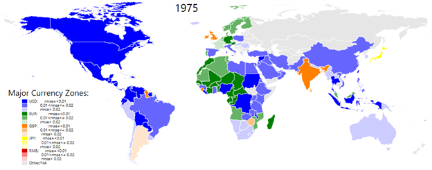
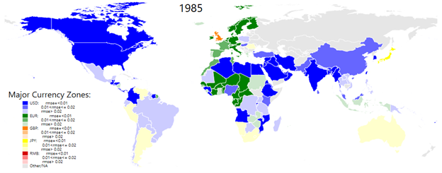
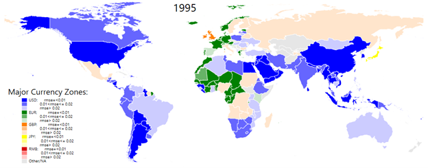
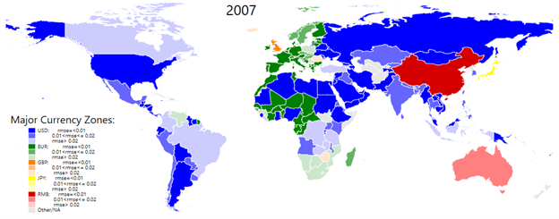
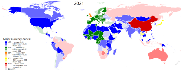
Figure 1: The Evolution of the Major Currency Zones. Source: Compiled by authors from their estimations.
In the map, each color is tinted in accordance with the level of the RMSE, which is categorized into three ranges of goodness of fit. An economy with a small RMSE (or a high degree of ERS) is represented in a dark color, while an economy with a large RMSE (or a low degree of ERS) is shown in a light color.
Painting each economy with a different color density increases the nuance of the analysis. Many researchers who have implemented the Frankel-Wei or Kawai-Pontines method have failed to incorporate the degree of the goodness of fit into the information. In other words, their approaches do not clarify whether the regression results have sufficiently high explanatory power or not.
Figure 1 contains several interesting points. First of all, the USD has been the most dominant anchor currency in the last five decades. In the aftermath of the collapse of the Bretton Woods system in 1973, major advanced economies have shifted to flexible exchange rate regimes, but many emerging & developing economies, except for some that pegged their exchange rates to former colonial powers’ currencies, decided to continue to stabilize their exchange rates against the USD. In the early 1990s, many of the former Soviet Union republics began to adopt the USD as their anchor currency.
Second, the EUR (or DEM before 1999) solidified its hold in Western Europe and spread eastward in the 1990s and 2000s. Economies in western and central Africa which had pegged their currencies to the French franc began to choose the EUR as their exchange rate anchor. However, outside the Euro Area, its vicinity, and western and central Africa, one does not observe the dominant presence of the EUR. Its sphere of influence is not comparable to that of the USD.
Third, the number of economies that have used the U.K. pound and/or the Japanese yen as anchor currency have been limited in the last five decades. By the mid-1970s, the number of economies that stabilized their exchange rates against mainly the U.K. pound had diminished. As of 1975, only Guyana, India, Ireland and Sierra Leone appeared to assign the highest weight to the U.K. pound among major currencies. As of 2021, virtually no economies use it in that way.
The Japanese yen also lacks its own sphere of influence. In 1985 when the Japanese economy was in its heyday, close to thirty economies (including Iran, Myanmar, Romania, Samoa, Singapore and Sweden) stabilized their currencies at least partially against the Japanese yen. Since then, the anchor currency role of the yen has declined, and in 2020 and 2021, about 20 economies and 7 economies respectively used the yen as a partial anchor.
Fourth, although in this analysis China is treated as a major currency country from 1999, the maps show only a few economies that belong to the RMB zone. Recently, many researchers have identified several economies as belonging to the RMB zone. However, most of such economies loosely stabilize their exchange rates against the RMB as indicated by the weak explanatory power of the estimation, i.e., the high values of the RMSE. As of 2021, several economies (including Australia, Botswana, Brazil, Colombia, Indonesia, Russia, and Uruguay) are identified as assigning the highest weights to the RMB as anchor currency among the major currencies. However, the RMSEs of these economies are high, so that their currencies are judged to be not closely tied to the RMB. If the goodness of fit were not considered, highly flexible exchange rate economies such as Brazil and Russia might be categorized as RMB-zone economies.
Ito and Kawai (forthcoming) also investigate what factors contribute to or prevent countries from belonging to each of the five currency zones. This exercise tests two hypotheses. The first hypothesis is that the weight of the currency basket is influenced not only by the structural characteristics of the economy, but also by trade, investment, and financial ties to the major reserve currency countries and regions (i.e., the United States, the euro area, the United Kingdom, Japan, and China). The second hypothesis is that the weights of the major currencies in a currency basket are determined by the shares of the major currencies in terms of other financial transactions. For example, The USD weight is influenced by the USD involvement in other types of financial assets, not just by trade, investment, and financial ties to the major reserve currency countries and regions.
Preliminary empirical analysis yields several interesting results.
First, the USD weight is positively affected by the share of trade with the United States and the US dollar shares in export invoicing and cross-border bank liabilities. Similarly, the EUR weight is positively affected by economies’ shares of trade with the Euro Area as well as the euro shares in export invoicing, inward FDI stock, and cross-border bank liabilities. The RMB weight is not greatly affected by shares of trade with, or inward FDI stock or borrowing from China. In sum, there are few statistically significant determinants of RMB weights.
These results provide evidence for the existence of network externalities. That is, countries with a high share of the U.S. dollar in trade, investment, and cross-border financial transactions, for example, tend to have a higher weight of the U.S. dollar in their currency basket, even if the country in question does not have close economic and financial ties with the U.S., and because of these externalities and network effects, the U.S. dollar will continue to play a dominant role in the international monetary system.
References:
Frankel, J., and S. J. Wei. 1994. Yen Bloc or Dollar Bloc? Exchange Rate Policies in East Asian Economies. In Macroeconomic Linkage: Savings, Exchange Rates, and Capital Flows, edited by T. Ito and A. Krueger. 295–329. Chicago: University of Chicago Press.
Ito, H. and M. Kawai. forthcoming. “Size of Major Currency Zones and Their Determinants,” RIETI Working Paper Series #XXX. RIETI: Tokyo.
Kawai, Masahiro and Victor Pontines. 2016. “Is There Really a Renminbi Bloc in Asia? A Modified Frankel-Wei Approach.” Journal of International Money and Finance, 62 (April), pp. 72–97.
So simple, even I can understand it, and yet still cleverly done. Bravo.
“These results provide evidence for the existence of network externalities.”
This is one way we know the authors are onto something. If their results didn’t demonstrate network externalities, we’d have a problem. Network externalities are likely a major cause of the inertia seen in currency dominance.
An interesting detail in the 2020 map – Mexico’s pesos has drifted from strong dollar dominance to weak euro dominance. Structural change or data anomaly?
That is curious, isn’t it? I looked up Mexico’s trade in 2021 at the Britannica website:
“The United States is Mexico’s most important trading partner, and U.S.-based companies account for more than half of Mexico’s foreign investment. The United States is also the source of between two-fifths and one-half of Mexican imports and the destination for some four-fifths of the country’s exports.”
The top EU country as a source of exports was Germany, at 1.5%.
I think I’d have to go with “if you test a lot of relationships, you’ll find at least a few spurious ones…”