Chair Warsh’s focus on the Fed’s balance sheet and inflation can be interpreted in many ways. One way is a money base version of the Quantity Theory.

Take the Quantity Theory as an identity:

MV = PQ

P = MV/Q

Let M = MB × mult, where M is a broad measure of money, MB  is the money base, roughly the liabilities side of the Fed’s balance sheet. Take logs, where lower case letters denote logs of upper case letters.

p = mb + log(mult) + v – q

One can think of q as a determinant of money demand, usually GDP, but could be “total transactions”. Omitting v, here’s a graph of the price level and money base to GDP:

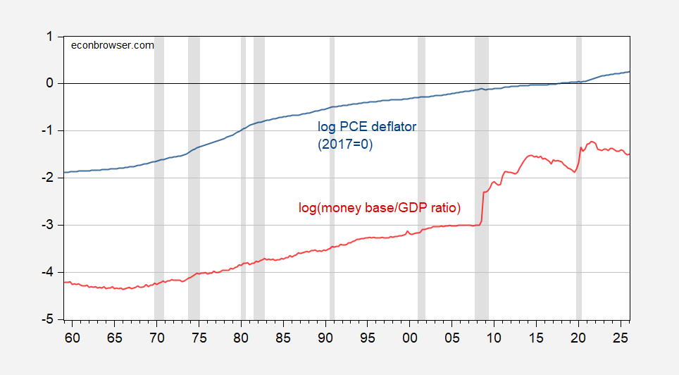
Not an obvious empirical relationship.

Take the first difference. If velocity and money multiplier are constant, then:

 π = Δmb – Δq

Maybe there’re short run and long run relationships implied by money base quantity theory (if I can coin a phrase). Then I estimate an error correction model imposing a 1:1 cointegrating relationship between money base and GDP, over the 1959-2019 period (so, ending before the pandemic-associated round of quantitative/credit easing).

 π_t = 0.000 -0.003mb_t – 0.003 Δq -0.0005(mb_t-1–q_t-1 ) + 0.008Δmb_t-1 + 0.016Δq_t-1 + 0.825π_t-1

Adj-R² = 0.73, SER = 0.0033, DW = 2.21, NObs = 242, bold denotes significance at 10% msl using robust standard errors. Differences above are not annualized.

The dynamic out-of-sample ex post forecast (aka historical simulation) shows that inflation is barely tracked.

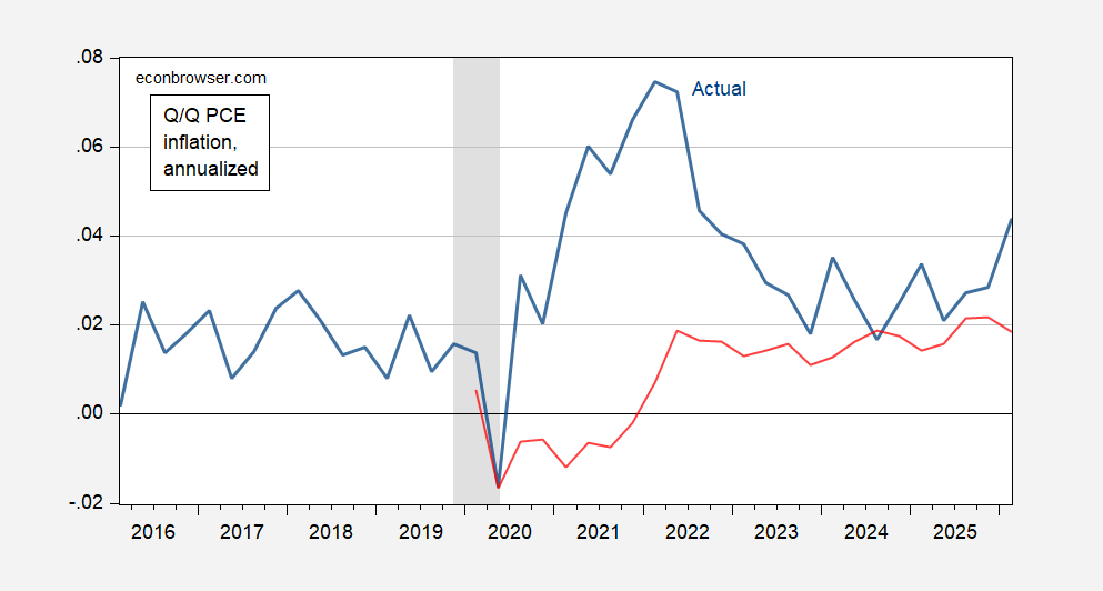
Figure 1: Q/Q annualized PCE inflation (blue), ex post simulation (red). NBER defined peak-to-trough recession dates shaded gray. Source: BEA, NBER, and author’s calculations.

There’s probably a specification that produces “better” predictions, but i don’t think there is one that does a lot better. That’s because the specification above, taking away the lagged inflation rate, has only a 12% adjusted R².