Reader Steven Kopits writes “potential GDP model is also a binding constraint model”, so GDP “…is subject to some sort of natural speed limit which cannot be exceeded”. This assertion is so amazingly absolutist in nature, and represents such a misunderstanding of how macroeconomists typically think of potential, that I am moved to observe that if this were so, output would never exceed potential GDP in our frameworks. Now, let’s consider the relevant depiction implied by the CBO estimates (using a production function approach [1]).
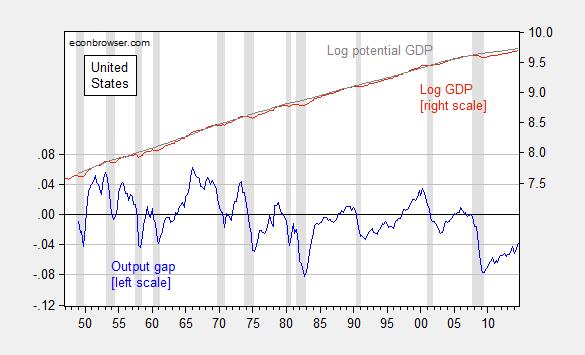
Figure 1: Log output gap (blue, left scale) and log GDP (red, right scale) and potential GDP (gray scale), all in bn. Ch.2009$, SAAR. NBER defined recession dates shaded gray. Source: BEA, 2014Q3 final release, CBO Budget and Economic Outlook (February 2014), NBER, and author’s calculations.
Note that output exceeds potential on numerous occasions according to CBO estimates, and hit 3.5% (log terms) as recently as in 2000. That’s because in this framework (the neoclassical synthesis, as forwarded in for instance Samuelson’s textbook, or e.g., here), factors of production can be utilized at greater than “normal” rates.
Now there are interpetations of potential GDP that fit Kopits’ description; from this post:
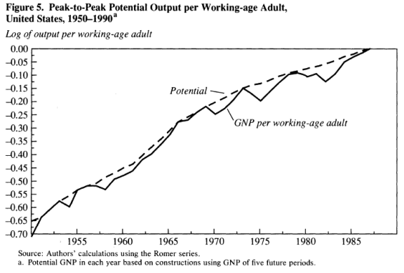
In Summers and Delong (1988), the authors provide an interpretation of potential as a level of output that can’t be exceeded (to me this is reminiscent of the Friedman “plucking model” (re-iterated in a 1993 publication, see also [1], [2])). Figure 5 depicts per capita potential under this interpretation.
Figure 5 from Summers and Delong (1988).
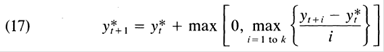
The formula used is given by recursive application of their equation 17:
Where y* is potential GDP, and k=3 to 5. It’s of interest to consider what an updated version of the De Long-Summers procedure implies for the output gap. I apply the procedure to log GDP instead of per working age worker, and set k=3.
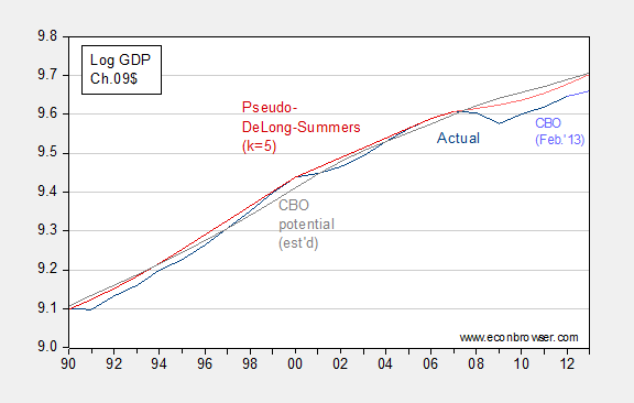
Figure 1: Log GDP (dark blue), CBO February 2013 projection (light blue), CBO potential, estimated by using 2011 ratio of 2009$ GDP to 2005$ GDP (gray), pseudo-DeLong-Summers (k=5) using actual data (dark red), and projection using CBO projections (pink). Source: BEA, CBO Budget and Economic Outlook (February 2013), and author’s calculations. [DeLong-Summers series calculation corrected 4:10pm]
As of 2012, the output gap using the DeLong-Summers (1988) procedure is quite similar to the implied CBO gap — 3.1% vs. 4.3% (log terms). There are a couple of caveats.
First, the CBO has not released an estimate of potential that is consistent with the newly back-revised BEA GDP series. Hence, I have resorted to the expedient of adjusting the CBO potential GDP series by the ratio of actual GDP in 2011, expressed in 2009$ and 2005$ from the respective series.
Second, since the calculation of the DeLong-Summers procedure requires values of future growth, one can only calculate the 2012 value using estimates of 2013, 2014 and 2015 growth. In the figure above, I use the CBO’s February 2013 projections. The upward movement in the potential GDP in 2013 (and later, not shown) is due to the projected surge in GDP growth in 2015 and 2016 (in excess of 4%). If one were to forecast tepid growth in those years, the trajectory of the pink line would be depressed with a commensurately smaller output gap, in absolute value. (Setting k=4 or k=3 would also yield a different set of estimates.)
So, the implied degree of policy activism one should pursue in 2013 could differ substantially depending on views of the evolution of potential. Note that in Delong and Summers (2012), potential is endogenous, depending on the level of current economic activity (hysteresis effects, etc.), providing an additional reason for pursuing activist macroeconomic (specifically, fiscal) policies.
In the context of the Summers-DeLong (1988) framework, potential does constitute kind of a speed limit (although not completely since higher investment can increase the capital stock and hence elevate the trajectory of potential). But this speed limit interpretation does not apply for case for the conventional interpretation of potential GDP I use. Still plenty of wide, open road, and no speed limit in sight in this view.
I wish people would read an intermediate (heck, maybe an intro) macro textbook before saying what’s in the textbook…
For more discussion of how macroeconomists typically interpret potential, see this post, and Weidner, Williams/SF Fed. Notice that if one uses Mankiw’s approach of inverting the Phillips curve, the output gap is about -5.75% (log terms), even taking into account the upwardly revised GDP growth for 2014Q3 in the final release.
“Potential” GDP is unknowable. You can swerve this in any way to fit a dialect.
You’ll know when we reached potential GDP when accelerating inflation fails to raise real GDP.
We’re a long way from potential output, in part, because of globalization and the Information Revolution.
Also, I may add, in 1999, we started hiring bag ladies and guys sleeping in the park from temp agencies to process paperwork.
We’re nowhere near that point.
This is an interesting take on potential GDP: https://growthecon.wordpress.com/2014/12/15/youve-got-potential/
Here’s another view:
http://upload.wikimedia.org/wikipedia/en/7/7e/U.S._Phillips_Curve_2000_to_2013.png
Well, let’s see how the CBO defines potential GDP:
“Potential output is an estimate of “full-employment” gross domestic product, or the level of GDP attainable when the economy is operating at a high rate of resource use. Rather than being a technical ceiling on production, potential GDP is a measure of the economy’s maximum sustainable output, in which the intensity
of resource use is neither adding to nor subtracting from inflationary pressure.”
And what of pGDP trend?
“The long-term trend in real (inflation-adjusted) GDP is generally upward (see Figure 1) as more resources—primarily labor and capital—become available and as technological change allows more-efficient use of existing resources.”
To me, that reads like “some sort of speed limit”. If GDP growth were unlimited or unconstrained, potential GDP would be a meaningless concept. (And it may be, in fact.)
http://www.cbo.gov/sites/default/files/03-16-gdp.pdf
Steven Kopits: Yes, I know that’s the CBO’s definition (I was a Fellow in CBO’s Macro Analysis Division, 2005). You can interpret potential GDP as a speed limit, but you’ll notice that if the Fed is willing to tolerate accelerating inflation over some period, then GDP can exceed potential in a noticeable fashion. So, it’s a very flexible speed limit (more autobahn than US interstate), and certainly not a hard constraint. And that was my point.
And I didn’t say it was a hard constraint. I said it was “some kind of speed limit.” It has to be for potential GDP to be a useful concept as a forward forecasting or policy tool.
But I don’t know Menzie. It does vary. Not a lot, but it does, and particularly during times of stress. It’s like ‘the speed limit is 55, unless it’s been raining or it’s really sunny.” If that’s true, then I really need a weather forecaster more than an economist, if you get my drift.
In any event, I saw the ‘natural rate’ as a virtue. If we take a binding constraint view, then oil has restrained growth. With that constraint removed for the moment, the gate should be open for accelerated growth to the next binding constraint. If I believe Larry Summers, it could be labor. And if that’s so, it suggests some pretty interesting dynamics coming up within a matter of months (several months). Put another way, if we take a binding constraint approach, and assume a rotation among constraints, then the easing of one constraint prompts us to undertake a search for the proximate constraint. In that sense, both a supply-constrained oil markets view, as well as the ‘natural rate’ aspect of potential GDP, help focus our investigations on key areas.
Steve Kopits: Well, that’s certainly more nuanced than what you wrote in your comment. Let me re-quote:
where “it” is GDP. I have edited the post to put in bold face the relevant text.
Of course, you are correct.
I should have written ““…it is subject to some sort of natural speed limit which cannot be exceeded sustainably”
You know, I am increasingly uncomfortable with long range forecasts. A forecast has value if it informs decision-making.
As you know, I crank out forecasts literally every day. I am well aware of the limitations of these. Frankly, you should see the knock-down-drag-out arguments we’re having one tab over with people with access to all the databases in the world and unparalleled experience. And yet even twelve months out is a huge battle.
Whenever I see a 2040 forecast from anyone–Exxon, EIA, or even myself–I cringe. Go back just five years and find me anyone–cornucopian or peakist–who even mentions shale oil. It’s just not there. And yet, today, it’s literally driving the global economy. If I believe some of the numbers I’m seeing, the US will be a major exporter within a handful of years. In any event, about five years out is as far I think I can reasonably project with any kind of confidence. After that, it’s really speculation.
So is potential GDP a useful concept? I think it’s helpful to think in terms of some kind of gap, and some kind of trajectory of that gap. But I don’t know. If that ‘natural speed limit’ is not that stable, then pGDP itself is not that useful, certainly not in the out years.
So, let’s see how much running room we have in front of us.
If we assume the 2007 CBO pGDP line is right, and convergence occurs by year-end 2018, then GDP would have to increase by 4.9% per annum on average. That’s a pretty tall order.
If we assume the CBO’s 2011 pGDP line is right, then convergence would occur in 2018 at a 4% average growth rate.
I think we’ll be somewhere in this range. If this interpretation is right, then we’ll see many more quarters of growth at rates seen in the last two. These will prove not an anomaly, but a harbinger of things to come. Indeed, during stretches, we might see growth rates not experienced in the US since, say, the Kennedy administration.
My post on this matter is here: http://www.prienga.com/blog/2014/12/28/regaining-potential-gdp
It should be noted, the U.S. offshored older industries, imported those goods at lower prices and higher profits, and freed-up a lot of U.S. labor.
Also, U.S. Information-Age firms, which became more efficient after the quick and massive “creative-destruction” process, mostly from 2000-02, earn high profit margins and are sitting on huge piles of cash (the U.S. not only leads the world in the Information Revolution, it leads the rest of the world combined, in both revenue and profit).
So, there’s plenty of unused labor and capital, or productive capacity.
Labor’s share is at a record low to GDP, which constrains labor productivity and growth of real, after-tax and -debt service purchasing power of the bottom ~90% (the spending of which makes up ~35-40% of GDP).
Debt to wages and GDP is at or near a record high, which results in total annual flows to the financial sector absorbing an equivalent of all annual economic output, i.e., “hyper-financialization”. The output of the US economy for the next 7-10 years or more is pledged to the financial sector, which by extension implies the top 0.01-0.1% to 1% of households who own a disproportionately large share of financial assets with the associated claim on labor, profits, and gov’t receipts indefinitely.
The record debt to wages and GDP coincides with record asset valuations to wages and GDP and thus the drag effects on growth from wealth and income inequality, which reduces money velocity and thus constrains, or precludes, the reflationary effect of reserve expansion and asset bubbles.
The Marxian decelerating rate of real, after-tax profit growth since 2000 and 2007 is associated with falling labor share to GDP and marginal productivity, as well as the decelerating rate of real GDP per capita since 2000 from 2.1% to below 1%.
Thus, hyper-financialization and asset bubbles are not a solution as the Fed (and TBTE bankers) implies (imply) but an unequivocal sign of peak and incipient decline.
If one examines the real aggregate cyclical change rate of growth of gov’t receipts less social insurance (spending less the fiscal deficit), profits after tax, and personal income, the implicit real final sales less the US gov’t deficit has decelerated to the “stall speed” that historically preceded, or coincided with, recessions.
The US economy is much closer to the historical “stall speed” and tipping point towards recession than most realize. The rolling over of housing, rising subprime auto loan delinquencies, and eventually the oil and shale boom/bubble investment, extraction, and employment will be a drag on industrial production and a prospective precipitant for at least a “growth recession” or “stall speed” in 2015.
Thus, expect to see gov’t spending as a share of GDP increase in 2015, along with the deficit as a share of GDP, not because gov’t spending increases but because GDP decelerates. The Fed will not raise the reserve rate in 2015 but instead likely resume QEternity sometime in 2015 by a similar monthly amount as during 2009-14 in order to fund the fiscal deficit to prevent nominal GDP from contracting in 2015-16. The consensus does not want this to be expected and internalized, as it implies that the US and the rest of the English-speaking world will follow Japan and the EZ, and we must tell ourselves over and again that “the US is not Japan”, no matter that the data clearly indicate that we are following precisely the expected trajectory in terms of CPI, yields, and the 5- and 10-year trend of real GDP per capita.
Remember, the yield curve DOES NOT INVERT during debt-deflationary regimes (Schumpeterian depressions) of the Long Wave Trough, and neither will the curve invert this time. Rather, the 10-year Treasury yield is more likely to decline to well below 2% to as low as 1% by the end of the decade, as the trend rates of CPI and nominal GDP decelerate to 1% or below and 2% or below respectively by the end of the decade or the early 2020s.
Because of hyper-financialization, the stock market is the economy, and a stock bear market cannot be permitted by the Fed and TBTE banks to occur or risk a contraction in net annual flows to the financial sector, which in turn would risk another 2008-09-like financial system meltdown and outright recession and contraction of nominal GDP.
Therefore, we have a system in which the largest commercial banks are effectively gov’t-sponsored hedge funds that cannot be permitted to fail, must be supplied with no-cost reserve liquidity to lever up equity index futures and to clear US gov’t debt, and thus no longer serve a productive intermediary role as suppliers of private credit for productive enterprise but are instead gov’t-sponsored, -enabled, and -protected extractive entities with little or no accountability except to one another.
Virtually no established economist can say this publicly or risk job, tenure, chairs, endowments, gov’t appointments, lucrative consulting gigs, and the like. Unfortunate but reality.