An Econometric Assessment of the World according to the American Legislative Exchange Council (ALEC)
For eight years, the American Legislative Exchange Council has been producing a ranking that purports to measure the competitiveness of individual states. From ALEC, Rich States, Poor States, 2015:
The Economic Outlook Ranking is a forecast based on a state’s current standing in 15 state policy variables. Each of these factors is influenced directly by state lawmakers through the legislative process. Generally speaking, states that spend less—especially on income transfer programs, and states that tax less—particularly on productive activities such as working or investing—experience higher growth rates than states that tax and spend more.
Hence I think it is reasonable to ask whether the ALEC-Laffer-Moore-Williams “economic outlook” ranking (hereafter “ALEC ranking”) actually has any predictive power, above and beyond other demographic and geographic indicators. This analysis follows up on a more ad hoc analysis in this post, and confirms conclusions arrived at in Fisher w/LeRoy and Mattera (2012). In addition, this analysis serves as a rejoinder to ALEC’s rebuttal asserting that critiques did not incorporate sufficient controls and allow for differing time horizons, to wit:
Moreover, rigorous statistical methods show that a higher economic outlook ranking in Rich States, Poor States does indeed correlate with a stronger state economy.
H/t Michael Hiltzik, who has done a tremendous job tracking the ALEC ranking. Let’s examine the available data.
Figure 1 depicts the one year growth in real Gross State Product and the ALEC ranking, lagged one year, for growth over the 2008-2014 period. Should the ALEC thesis be correct, one should see a negative sloped relationship.
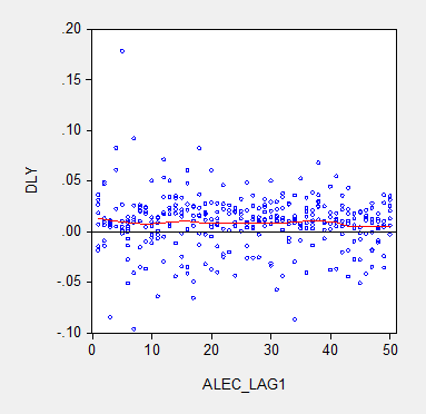
Figure 1: Real Gross State Product growth (log first difference) and lagged ALEC ranking for Economic Outlook. Nearest neighbor fit line (red), window = 0.3. Source: BEA and ALEC, Rich States, Poor States, 2015, and author’s calculations.
There is no obvious correlation between annual growth rates and the ALEC rankings. Note that lagging the ranking so that, for instance, the growth rate between 2013 and 2014 is related to the ALEC ranking in 2012 (instead of 2013) does not change the results much. (The ALEC 2013 ranking pertains to data reported in 2012, as far as I can tell). This outcome is unsurprising because the ALEC rankings are highly persistent. If one estimates a panel autoregressive model for the ALEC rankings, the AR coefficient is 0.95, and the adjusted R2 is 0.90.
Defenders of the ALEC rankings have argued that the rankings are aimed at predicting growth at a longer time horizon than annual. Given that the perspective of the RSPS methodology is supply-side, this argument is prima facie sensible. In order to accommodate that argument, I display in Figure 2 the data for three year (nonoverlapping) horizons (for 2014, and 2011).
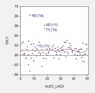
Figure 2: Nonoverlapping average three year real Gross State Product growth (log difference) and three year lagged ALEC ranking for Economic Outlook. Nearest neighbor fit line (red), window = 0.3. Source: BEA and ALEC, Rich States, Poor States, 2015, and author’s calculations.
Figure 3 provides analogous information, at the six year horizon (the maximum possible given the span of ALEC rankings).
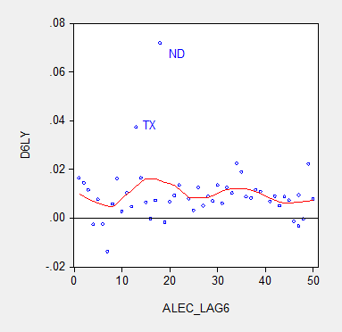
Figure 3: Average six year real Gross State Product growth (log difference) and six year lagged ALEC ranking for Economic Outlook. Nearest neighbor fit line (red), window = 0.3. Source: BEA and ALEC, Rich States, Poor States, 2015, and author’s calculations.
The nonparametric fitted lines indicate a slightly negative slope overall, suggesting some content to the argument that lower ranked states grow slower. In both Figures 2 and 3, North Dakota and Texas constitute outliers along the y-dimension. In order to discern how much these two observations drive the results, I omit them and replot in Figure 4.
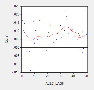
Figure 4: Average six year real Gross State Product growth (log difference) and six year lagged ALEC ranking for Economic Outlook, excluding North Dakota and Texas. Nearest neighbor fit line (red), window = 0.3. Source: BEA and ALEC, Rich States, Poor States, 2015, and author’s calculations.
No obvious pattern emerges from this last plot. In order to move beyond simple graphics, I now implement a series of regressions. First to a simple examination of the a bivariate relationship, encompassing the lower 48 states, one obtains at the annual frequency:
Δyi,t = -0.00003ALECi,t-1
Adj-R2 = -0.00, SER = 0.027, N=288. bold indicates significance at 10% msl, using heteroscedasticity and serial correlation corrected standard errors.
(I use the lower 48 as I do not have demographic and geographic data for the Alaska and Hawaii.)
Essentially, there is no explanatory power for the ALEC-Laffer indices in terms of year on year GSP real growth. Allowing for individual state-fixed effects, one obtains:
Δyi,t = 0.0004ALECi,t-1
Adj-R2 = -0.00, SER = 0.027, N=288. bold indicates significance at 11% msl, using heteroscedasticity and serial correlation corrected standard errors.
The coefficient is positive, indicating that lower ranked states, and hence states that have a less business friendly environment according the ALEC criterion, exhibit higher economic growth. The coefficient is borderline statistically significant. I would say that the use of state-level fixed effects is a fairly blunt way to account for state-specific factors. A better approach controls for state factors that economic theory suggests might be important for growth, such as geographic and demographic factors. Here we include log population density (LDENSITY, to account for urbanization), dryness (measured as inverse, WET), mildness of weather (MILD) and proximity to navigable waterways (DISTANCE); these four variables are defined such that positive coefficients are expected. These variables are time-invariant; hence one cannot estimate a fixed effects regression incorporating these variables. I also include log real price of oil (LRPOIL) to control for oil producing states, allowing the coefficient to vary across states.
Δyi,t = 0.0002ALECi,t-1-0.01LDENSITYi + 0.019WETi + 0.001MILDi + 0.0001DISTANCEi + LRPOILi,t
Adj-R2 = 0.36, SER = 0.021, N= 288. bold indicates significance at 10% msl, using heteroscedasticity and serial correlation corrected standard errors.
The ALEC ranking has no statistical significance, while a drier and more mild climate is associated with faster growth, with statistical significance. Proximity to navigable water is also a positive factor.
What if we estimate a comparable regression, looking at 6 year growth rates (but omitting oil prices which are the same for all states)? Then one obtains:
Δyi,t = -0.018 -0.0001ALECi,t-6 +0.001LDENSITYi – 0.0007WETi – 0.0003MILDi -0.00001DISTANCEi
Adj-R2 = -0.02, SER = 0.007, N= 48. bold indicates significance at 10% msl, using heteroscedasticity and serial correlation corrected standard errors.
Notice that the ALEC coefficient is not statistically significant. Thus far, the one case it has shown up as borderline significant, it goes the opposite of the ALEC-Laffer-Moore-Williams thesis.
Finally,Professor Ed (“no recession”) Lazear recently asserted that states with fast growing employment have low tax rates and right-to-work laws. He also argues that one needs to incorporate the depth of the drop in employment in 2008-09, in order to explain the growth in employment (so, a sort of version of the bounceback thesis he forwarded in the Economic Report of the President, 2009). I can’t find the working paper that provides the basis for his assertion, but I can estimate a comparable regression. In order to make the proposition testable, I examine 5 year growth rates in output, and refer to the ALEC rankings in 2009. I add the change in output from 2008 to 2009 (so TROUGHDEPTH takes on a value of -0.05 for observation i if output dropped 5% going into 2009).
Δyi,t = 0.065 -0.0010ALECi,t-5 +0.0046LDENSITYi + 0.0042WETi – 0.0014MILDi +0.00005DISTANCEi – 0.3413TROUGHDEPTHi
Adj-R2 = -0.04, SER = 0.037, N= 48. bold indicates significance at 10% msl, using heteroscedasticity corrected standard errors.
The ALEC variable does not exhibit statistical significance. Omitting ND and TX would not change this basic results. Moreover, the trough variable coefficient, while exhibiting the right sign, is not statistically significant.
Bottom line: The ALEC ranking, which purports to measure business-friendly policies, is not correlated with real GSP growth, either short term or medium term. This is true if one controls for additional variables.
I don’t think this necessarily means that policies such as right to work, or tax rates, and so forth do not have an impact on growth. For instance, Kolko, Neumark, and Cuellar Mejia, J.Reg.Stud. (2013) conclude that what’s important is “less spending on welfare and transfer payments; and more uniform and simpler corporate tax
structures.” Hence, the ALEC economic outlook ranking is, in my assessment, a manifestation of faith based economics.
Addendum: As Wisconsin has risen in ALEC rankings (33rd in 2008 to 17th in 2014), Wisconsin’s growth rate has declined relative to the US.

Figure 5: Wisconsin-US real growth differential (log first difference) and lagged ALEC ranking for Economic Outlook for Wisconsin (down is a “better” ranking). Light green shaded area pertains to GDP growth rates during the Walker era. Source: BEA and ALEC, Rich States, Poor States, 2015, and author’s calculations.
If it is not obvious, this is not the direction that ALEC-Laffer-Moore-Williams posit.
Note: Thanks to Professor Neumark, who kindly provided the data set used in his J.Reg.Stud. paper for use by my students in my PA819 statistics course (all students had to use his data set to analyze whether business conditions as measured by various indices (but not the ALEC ranking) influenced state level growth). The demographic and regional variables are drawn from that data set.
” . . . a manifestation of faith based economics.”
One must have faith in the economics of Foxy Noise promotion and Koch Bro funding.
Logically it seems like this is a bad result for liberals and a good result for economic conservatives. If there is no difference in growth between states with high taxes and those with low taxes than policymakers might as well let people who earn money keep as much of that money as possible (e.g. have very low taxes), right? I mean, this shows that economic growth will be the same, right? So be fair and let the earners keep their money!
Anon, perhaps, and it would be that much more instructive to discern the sources of private and public investment as a share of wages and gross state product, transfers per capita, employment, wages, real, after-tax purchasing power, distribution of same, and the sectors that predominate, including relative share of tradable flows.
As for “earners”, the US is now experiencing earned income (from wages and salaries for the bottom 80-90%) as a share of GDP at a record low, as well as capital formation as a share of GDP at the level of 20-25 years ago while FINANCIAL (non-productive, speculative rentier) capital, i.e., debt and asset values as a share of wages and GDP and associated rentier claims in perpetuity, is at a record high.
In fact, annual net flows to the financial (and financialized sectors of “health” care and “education”) sector and its top 0.001-1% owners now equals 100% of annual value-added (GDP) output of the US eCONomy.
To relate that publicly (or worse, to internalize it personally at existential professional risk) is a lot to ask of an eCONomist of any ideological stripe and predisposition, especially s/he with Establishment standing; a six- or seven-figure income and mortgage; annual mid-five-figure private school tuition for offspring; a beach house away from the riff-raff; annual property taxes equaling, or exceeding, the US median household income; leases on European luxury vehicles that amortize to as much, or more, than the typical working-class person earns after inflation and taxes in a lifetime; and a female spouse’s physiological cosmetic adjustments of various kinds; it might reveal biases AND so much more that society needs to know to inform policies that benefit the vast majority of us. WHAAA?! GASP!!!
But this writer is biased in that way. Forgive me (don’t you dare).
Anonymous Very clever, but I don’t think your argument holds up. For one thing, every dollar that an “earner” gains in lower taxes is also a dollar that some other “earner” loses due to an offset in state expenditures. You have slipped in the hidden assumption that state expenditures add no value and therefore the recipients of those expenditures are not “earners.” As one of my old profs used to say, this is just another version of Marx’s labor theory of value. And it is.
But the bigger problem with your post is that it assumes liberals argue for higher taxes on the grounds that higher taxes increase economic growth. I don’t think that’s the liberal rationale for higher taxes, so the fact that there is no statistically significant difference between high tax and low tax states does not undercut a liberal argument for higher taxes. There are several good reasons for higher taxes. First, higher taxes on the wealthy allow income redistribution towards lower income folks. Contrary to what most rich folks like to believe, they did not “earn” their money all on their own. Most of one’s earnings are due to dumb luck; e.g., birth, state of the business cycle when entering the labor force, genetics, family and friend networks, etc. On fairness grounds I don’t think we want to reward good luck and punish bad luck. Second, higher tax rates in the form of higher estate or inheritance taxes fight income inequality and political inequality. And oh by the way, there is plenty of evidence that high inheritance taxes encourage greater workforce participation, which is good for economic growth. Finally, and this is really the heart of the matter, we want higher taxes because they tend to increase total welfare even if that higher welfare doesn’t show up as higher observed GDP/GSP. This is because public goods tend to generate a lot more consumer surplus than private goods; and this is because individual demand curves for public goods are summed vertically while individual demand curves for private goods are summed horizontally. This means public goods, which are evaluated at the cost of providing the good tend to understate their true welfare value because so much of the consumer surplus is unobserved and unmeasured. Let me give you an example. In GDP and GSP accounting the value of crime fighting is evaluated by summing the costs for police, courts and prisons. But the value to the community is almost always much higher even though no one person would be willing to pay for 100% of the cost.
I think, people are willing to pay. For example, I heard realtors say people are willing to pay an extra $50 a square foot for a house in a good school district. For a 2,000 square foot house, that’s an extra $100,000. Also, they’re willing to pay several thousand dollars more for a house with parks or open spaces nearby.
Peak Trader I think you misunderstood the example. Being willing to pay more to live in a safer area is not an example of a public good. The public good is in reducing crime, which is very different from moving away and shifting the burden of crime onto someone else. If everyone paid and extra $100K towards crime prevention the welfare benefits of lower crime rates would dwarf the private benefits of moving to a different district. Again, remember the geometry of public goods versus private goods. With public goods the benefits are summed vertically; with private goods the benefits are summed horizontally. In general the welfare triangle of the former is greater than the latter.
2slugbaits, if you want to live in a safer area, or make your area safer, you have to pay for it. Public goods don’t materialize out of thin air. People have different values. That’s why all communities aren’t the same.
The values of a community go a long way to explain the state of the community.
How does ALEC ranking correlate with GSP level ?
It seems to be that – as with countries – convergence should be the default expectation , thus you would need to correct for levels/catch-up growth in your regressions.
IF ALEC biases their high ratings to low GSP level states , they may achieve average growth rates only because of an underlying catch-up premium , meaning that ALEC-favored policies actually do hurt growth.
Marko: Forgive me, but I thought the convergence literature had settled on convergence clubs, rather than a single level. I suspect the same is true for the US. But in any case, if I incorporate initial level relative real per capita in the six year regression, there is essentially no change in the results.
Yes, I see now that the evidence for convergence clubs is pretty strong , and that certainly complicates the matter. Good to know that initial level gdp makes no difference , in any case. Thanks.
BTW , I found this recent paper revealing on the relative performance of the “clubs” :
http://wweb.uta.edu/faculty/cychoi/Research/EI(2015)%2049-71.pdf
P.S. When I said ” It seems to be ….” , above , I meant to type ” It seems to me….” , so that may have given the impression that I knew more about state level gdp dynamics than is actually the case.
Menzie, ALEC is a Chicago school right-wing propaganda think tank, but it’s nice that you have supposed they are unbiased. Seems you had a couple of hours left, for some statistical work.
John: I need to demonstrate these points for the “true believers”. I admit it took a little time — but most of the effort was typing the ALEC rankings into the computer. The statistical analysis is intro stats, so that part took very little time.
Given states have to balance their budgets, cutting taxes requires spending cuts, which isn’t a stimulative policy on GSP. However, I’d expect the mix of GSP to change.
I’d expect education to be a significant factor, because many new jobs are higher skilled jobs.
And, on a national level, the output gap – measured by per capita real GDP – hasn’t begun to close, except through the destruction of potential output, even with accommodative monetary policy and stimulative fiscal policy.
It’s a very unusual period, because the country is still in depression, after the severe recession.
Not on subject, I know — but did you read about Stephen Moore’s backtracking on an alleged phone call with Scott Walker?
First he reported a phone conversation with Walker during which Walker stated a particular position on immigration.
Now Moore is saying the phone call never actually took place!
Whoops, forgot to share the link with you: http://www.nytimes.com/politics/first-draft/2015/07/06/forget-what-i-said-that-scott-walker-call-never-happened/