Commenting on the Kansas Palmer Drought Severity Index, Rick Stryker writes: “From a theoretical point of view it must be stationary.” He reasons that this is so, because it is bounded between -10 and +10. Question: Is this a relevant piece of information when examining finite samples? Let’s look at consumption as a share of GDP, which must be bounded between 0 and 1.
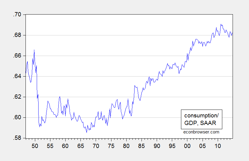
Figure 1: Nominal consumption to GDP ratio, SAAR (blue). Source: BEA, author’s calculations.
I retrieve the latest vintage of national income and product accounts, and apply the unit root tests readily available to me (ADF, DF(GLS), Phillips-Perron, Elliott-Rothenberg-Stock point optimal, and Ng-Perron), constant and trend. Using default settings, all fail to reject the unit root null. Applying the Kwiatkowski-Phillips-Schmidt-Shin test, the trend stationary null is rejected. The results are here. The conclusions are unchanged if the specifications involve only constants.
Truncating the sample so as to start in 1952 (thereby omitting the high consumption ratio at the beginning) does not change the conclusions.
Now, it is true that consumption-to-GDP cannot stray outside the 0-1 bounds. But in a finite sample, the series might look a lot like a random walk. (Perhaps Rick Stryker, like the HeeChee, has access to the infinite sample, in which case he can find out for sure what the time series characteristics of the consumption-GDP series is.)
Menzie,
Let me explain a little further then.
The fact that the Palmer Drought Severity Index (PDSI) is bounded tells you something about the nature of the series itself. It’s standardized index of how dry or wet the environment is. It has to be bounded because the environment can only get so dry or wet. But, importantly, an index like that must be mean reverting given what it’s actually measuring. Sometimes it rains and it gets wetter. Then the rain stops and it drys up. But it never goes too long before it rains again. Atmospheric moisture in the atmosphere fluctuates. There is a water cycle. If all that weren’t happening, we wouldn’t be talking about this since there wouldn’t be any life.
The nature of a variable such as the PDSI is that we’d expect it to be stationary, although we’d want to confirm with the appropriate statistical test. As I pointed earlier, because you were estimating ECMs and using Johansen, it’s very easy to mispecify such a model by coming to a false conclusion about non-stationarity in the first stage. In econometrics, I believe that it’s important to bring any additional information you have to bear, whether formally in a Bayesian analysis, or informally in classical statistics. Given that we’d expect this variable to be stationary, it makes no sense whatsoever to rely on the ADF test statistic. There are only 45 data points and the ADF (and tests like it that have non-stationarity as the null) have very low power in small samples. If you are pretty sure the defendant is innocent, why would you put him in a legal system in which he’s presumed guilty and then set a very high bar for acquittal? If you are wrong and the defendant is innocent, you have mis-specified your model.
KPSS is a natural test in such a situation because it assumes that the series is stationary unless the data argue to the contrary convincingly. As I’ve already mentioned in previous comments, the reasonable assumption to make when applying this test is that the series is non-trending. When I run that test with the standard Bartlett kernel, I’m not even close to rejecting the null of stationarity at the 10% level, whether I use the Newey-West bandwith the software you use (eviews) prefers or whether I use the longer bandwidth I prefer to control better for oversizing of the KPSS test in finite samples. Failure to reject is robust as I have mentioned with the less frequently used Parzen and Quadratic Spectral kernels and for a range of bandwidths.
You’ve introduced a new term, “borderline rejects,” for cases when you can’t reject at the 10% level but you can reject at some lower unspecified level, and have partially justified your results using this concept. Of course, normally you can’t measure “borderline rejects” since papers and software packages generally tabulate critical values from 1% to 10%, assuming that no one would be interested in anything else. The KPSS paper computes critical values for the test statistic for the percentiles 1%, 2.5%, 5%, and 10% and software packages generally use the results published in the KPSS paper for their implementations of the KPSS test. I wondered what “borderline rejects” means in this case so just for fun I decided to extend the table of critical values for the KPSS test.
The standard critical values of the upper tail percentiles are reported in table 1 of Kwiatkowski et al in “Testing the Null Hypothesis of Stationarity Against the Alternative of a Unit Root.” Journal of Econometrics, 1992. The distribution of the test statistic is given by equation 14 in that paper, which I re-estimated by monte carlo simulation in order to extend table 1 in the paper. The critical values in the 1% to 5% range are a little different from what’s in table 1 since I’ve estimated them more accurately.
1% 0.743
2.5% 0.580
5% 0.461
10% 0.347
15% 0.284
20% 0.240
25% 0.211
30% 0.184
For the PDSI series, I can reject the null of stationarity at about the 29% level level then. That’s what “borderline rejection” means in this case. That may be enough for you to claim the PDSI is nonstationary but it’s not enough for me. I think your argument that Ironman estimated a spurious regression is false. As I said, he may have estimated a non-stationary against a stationary variable but that’s not clear either, given the mixed evidence on the agricultural output variable I discussed in the other post. I continue to think the results you reported are misspecified.
Rick Stryker: I was using specification with trend, obtaining test stat of 0.10. Critical value is 0.119.
Menzie,
Let me followup up on my comment I left on this post yesterday to more fully respond to your point.
We know from a theoretical point of view that a difference stationary process can be approximated arbitrarily closely by a trend stationary process and vice versa in finite samples. You don’t need to do a battery of unit root tests to establish that point. The consumption as a share of GDP series could be stationary with a near unit root but practically speaking behaves like its non-stationary in finite samples.
It’s also true that the reason we rely on asymptotic distributions is not because we are the HeeChee but rather because we hope that they are a good approximation to the finite sample distribution given the sample size we have and we want that approximation to get better as we add more data. If a trend stationary process is close to a unit root process in finite samples, treating it as if it were a unit root is not necessarily bad. We have some monte carlo evidence that the asymptotic distributions consistent with a unit root process are better approximations of the finite sample distribution even though the true process is stationary, e.g., the articles by Evans and Savin in Econometrica, early 1980s.
But that’s not the case here for the PDSI data. The time series tests don’t back up a claim that in finite samples the PDSI behaves as if it has a unit root. And we have a reasonable prior on this.
Menzie,
I left another comment on this last night. Did that get lost?
Rick Stryker: Just behind in approving. All up to date now.
Thanks Menzie.
My default, in this type of situation, would be to estimate an ECM with log consumption and GDP (or maybe GDP ex Consumption) and then use those to forecast the share if I need it.
I’ve been skeptical of shares of things in regressions for some time. It becomes most obvious if you do things like posterior predictive checks. For instance, if you fit an AR model to the above series and forecast it, you will get distributions that violate the constraints if you forecast long enough. It implies some kind of model misspecification. If you stick with a simple AR model, then the residuals should no longer be approximately normal if you hit high or low values for the series. You would instead be dealing with some kind of normal distribution with bounds that change over time.
Another possibility is omitted variables, which seem to be a problem here. When interest rates were high in the 70s, then I would expect the consumption ratio to be lower than normal. Alternately, there has been a significant decline in government spending as a percent of GDP, largely driven by defense spending. The model is not accounting for these exogenous changes.
All this talk about shares reminds me of stochastic portfolio theory. The interesting thing about stochastic portfolio theory is that it also thinks about the distribution of weights of the market portfolio over time. So for instance, in order for the market portfolio not to be dominated by a particular stock, there would be restrictions on the underlying price process.
Just an observation: stationarity implies that the statistical structure of the data is time-invariant. Boundedness does not imply such invariance.
“But, importantly, an index like that must be mean reverting given what it’s actually measuring. Sometimes it rains and it gets wetter. Then the rain stops and it drys up. But it never goes too long before it rains again.” — You assume climate is time-invariant. I sure wish this were true — mean dryness can shift over time.
DH,
Yes, mean dryness can change over time. The question is whether we have any good evidence that this is happening over the short time scales we are talking about–11 years– and whether, if mean dryness is changing, it is a large enough effect to be perceptible in the data.
The Intergovernmental Panel on Climate Change (IPCC) has provided analysis of their near-term expectations, i.e., out to 2050, in their recent 2013 report. Climate models do project changes in annual mean shallow moisture, with decreases in some geographical areas and increases in others. The same is true for runoff. However, the IPCC report does acknowledge that the hydrological models built into climate models are simple and so there is high model uncertainty. They label their projections “low confidence.” The report also emphasizes that natural variability tends to dominate in changes in the water cycle over this time horizon, which is about 35 years in their projections. We are talking about a decade of data in the PDSI index though.
Thus, a priori, we don’t have good evidence for changes in mean dryness over short horizons and we wouldn’t expect the effect to be large if we did. The KPSS test confirms that expectation.