As the administration pushes for “stability” in the Chinese exchange rate while imposing tariffs on China, it might be useful to recount the various ways in which different observers define currency “misalignment”. Here I update a primer first posted in 2010.

Currency misalignment can be determined on the basis of the following criteria or models:

• Relative purchasing power parity (PPP)
• Absolute purchasing power parity
• The “Penn Effect”
• The behavioral equilibrium exchange rate (BEER) approach
• The macroeconomic balance effect
  
• The basic flows approach
• An equilibrium approach

I have discussed several of these approaches in the past [0] [1], but a review of the approaches bear repeating, if only because there so much confusion regarding what constitutes currency misalignment.

Relative PPP

Relative PPP can be expressed as:

s = μ + p – p*

where lowercase letters denote log values, s is the price of foreign currency, p is the price index, and * denotes a foreign variable, and μ is a constant arising from the fact that p and p* are indices.

Using this criteria, a currency is misaligned if s deviates from the μ + p – p*. One difficulty is that μ has to be estimated. Typically, estimates of μ can vary drastically with sample period. Oftentimes, there is a time trend in q ( which equals s – μ – p + p*), which means that relative PPP cannot literally hold. Then, one might have to allow for a (ad hoc) time trend, which itself has to be estimated. In Chinn (Emerging Markets Review, 2000), I apply this approach to the East Asian currencies, pre-crisis.

In the case of China, presented below is the (log) trade weighted real effective exchange rate of China, (q), using the latest data spliced to an older series incorporating the swap rates pre-1994 per discussion in Chinn, Dooley, Shrestha (JIMF, 1999). Upwards denotes depreciation.

Using a simple linear trend, one obtains the counter-intuitive result that the RMB is overvalued. This suggests caution.

For more on effective exchange rates, see this survey paper (Open Econs. Review, 2015).

Absolute PPP

Given the drawback of relative PPP, it seems like one could get around the problem of estimating μ by using actual prices of identical bundles of goods across countries, rather than price indices.

s = p – p* or equivalently p = s + p*

where lowercase letters denote log values, s is the price of foreign currency, p is the price level, and * denotes a foreign variable.

The problem is that prices of identical bundles of goods are not collected. One thing that comes close is the Big Mac — hence the MacParity measure. But the problem is that prices of Big Macs (when expressed in a common currency) are systematically lower in lower income countries, and systematically higher in higher income countries. This is true when using Big Mac prices [2] [latest estimate] Parsley and Wei (2005) and when using the “price levels” in the Penn World Tables. This is so much a stylized fact that it is sometimes called “The Penn Effect”.

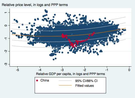
The Penn Effect

Instead of viewing the “Penn Effect” as a problem, one can exploit this stylized fact. Define r ≡ p – s – p*. Then one can exploit the relationship:

r = α ₀ + α ₁ (y-n)

Where y-n is log per capita income. In Cheung et al. (2008), we exploited this relationship (following Frankel (2005), in a panel regression setting. In that study, we found an approximate 40% RMB misalignment (in log terms).

In more recent work, we have adapted the analysis to incorporate nonlinearities (following Hassan, JIE 2016). In Cheung, Chinn and Nong (IF, 2017), we exploit the significant nonlinearity (a quadratic in per capita income) to find that as of the most recent data, China’s currency is not significantly undervalued, and plausibly is overvalued.

The Behavioral Equilibrium Exchange Rate (and related) Approach

Yet another approach is to use some theoretically and empirically motivated equations to estimate an exchange rate relationship. The variables can include productivity variables, or relative price of nontradables, or fiscal variables like the deficit, or interest differentials. Typically the variables can be motivated by some model of the exchange rate; which ones are included are motivated by goodness of fit. Goldman Sachs and JP Morgan had models of this sort. Zhang (China Economic Review, 2001) and Wang (2004) in Prasad (IMF, 2004) are some models in the public domain (see this 2007 Treasury occasional paper). Chinn (RIE, 2000) implements a specific type of BEER (or productivity based) model for East Asian exchange rates, while Ricci, Milesi-Ferretti and Lee (JMCB, 2013) examine a broader set of currencies. Chong, Jorda and Taylor (IER, 2012) look at long run income/exchange rate relationships (see this post).

A comprehensive set of estimates, updated regularly, is undertaken by Couharde et al. (EQCHANGE, described in this post).

The Macroeconomic Balance approach

The Macroeconomic Balance approach takes the perspective from saving and investment rates (see Peter Isard’s survey). Recall:

CA ≡ (T-G) + (S-I)

In other words, the current account is, by an accounting identity, equal to the budget balance and the private saving-investment gap. This is a tautology, unless one imposes some structure and causality. One can do this by taking the budget balance as exogenous (or use the cyclically adjusted budget balance), and then include the determinants of investment and saving. Then one obtains “norms” for the current account. Chinn and Prasad (JIE, 2003) is one example of this approach.

Then, using trade elasticities, one can back out the real exchange rate that would yield that current account. If that exchange rate is stronger than the actually observed exchange, then that currency would be considered “undervalued”.

Variations in this approach are numerous. One important question is whether to take official sector intervention as an exogenous (or somewhat exogenous) variable; doing so can yield a substantially different estimate of the normal current account balance, and hence equilibrium rate, as noted by Bayoumi, Gagnon and Saborowski (JIMF, 2015).

Starting in 2011, in a project I was somewhat involved in, the IMF began a process of revamping the approach. The External Balances Approach (EBA) emphasized desired policy factors such as social spending, and used annual data (see post here). The current formulation is embodied in the IMF’s External Sector Report.

The closely-related Fundamental Equilibrium Exchange Rate (FEER) determines the current account norm on a more judgmental basis (in other words, the current account norm is not estimated econometrically, just imposed per the analysts priors).

The Basic Balance approach

One could take a more ad hoc approach, asking what is the “normal” level of stable inflows — for instance looking at the sum of the current account and foreign direct investment, and see whether that value “made sense”. Or one could look at the sum of the current account and private capital inflows. If either of the flows are “too large”, then the currency would be considered undervalued (since a stronger currency would imply a smaller current account balance).

Note that a target value of zero for the current account or the basic balance is arbitrary, and does not in itself make sense. It behooves the serious analyst to remember this when considering, for instance, the Coalition for Prosperous America’s study.

It is interesting to make two observations. First, note the need for many non-model based judgments. To see this point, recall the balance of payments accounting definition:

CA + KA + ORT ≡ 0

Where CA is current account, KA is private capital inflows, and ORT is official reserves transactions (+ is a reduction in forex reserves).

Saying CA + KA is too big is the same, then, as saying ORT is too small, i.e., reserves are rising “too fast”. Morris Goldstein and Nick Lardy are among the most prominent exponents of this approach (see e.g., this this small volume).

Alternatively, running surpluses that are “too large” for “too long” will lead to foreign exchange reserves that are “too large”. Obviously, a lot of judgment is necessary here.

Second, one aspect of this judgment is that it is conditional on the constellation of all other macro policies, including monetary, fiscal and regulatory, in place. If the CA+KA is adjudged to be “too large”, one could say the exchange rate is “too weak”, but one could say with equal validity that the fiscal policy is “insufficiently expansionary”.

A (newer) Equilibrium View

The final approach would be to step back and think in terms of “equilibrium” exchange rates. One might argue that the exchange rate is undervalued if, in the absence of central bank intervention, the exchange rate would be stronger. Of course, this means that whenever any  central bank pegs an exchange rate, then the exchange rate is definitionally misaligned. I suspect when people use this particular definition, it is usually conjoined with some sort of threshold. One problem in my mind with operationalizing this definition is figuring out what that the right “threshold” is.

A more fundamental conception of what an “equilibrium” exchange rate is is laid out by my colleague Charles Engel. As noted in this post, the equilibrium exchange rate is the one that minimizes the distortion from sticky prices and other rigidities. That is not necessarily the exchange rate delivered by a free float, even in the absence of capital controls. Indeed, it might be best delivered by some type of monetary policy (see the paper).

This approach departs from the “equilibrium” approach embodied in the real models of the late Alan Stockman, as summarized here, in that those models assumed away nominal rigidities. With complete markets, the free floating exchange rate is almost irrelevant since the real rate will always adjust to the “right” levels.

Review and Summing Up

Two last observations. First, each of these approaches has advantages and disadvantages. PPP and variants are easy to implement, but are more akin to parity conditions, so it’s not clear over what horizon they apply to. The macroeconomic balance and FEER approaches are most appropriate to the medium term, and hence perhaps more relevant to policy questions. But they require more judgment on the parameters of the models. Moving to the basic balance approach, the time horizon is the shortest, and of perhaps most interest to policy analysts, and yet requires the greatest subjective judgment, since one needs to take a strong stand on what constitutes the appropriate values for critical variables. (There are also data considerations as well — the PPP criteria is most popular in part because of the limited data requirements.)

Second, in some ways, it’s not necessarily correct to think of these approaches as all inconsistent (in some instances they might be). Better to think that some approaches are more appropriate at one horizon versus another horizon. (This echoes Richard Cooper’s description of how elasticities, absorption and monetarist interpretations were all consistent over time, in thinking about the effects of devaluations.)

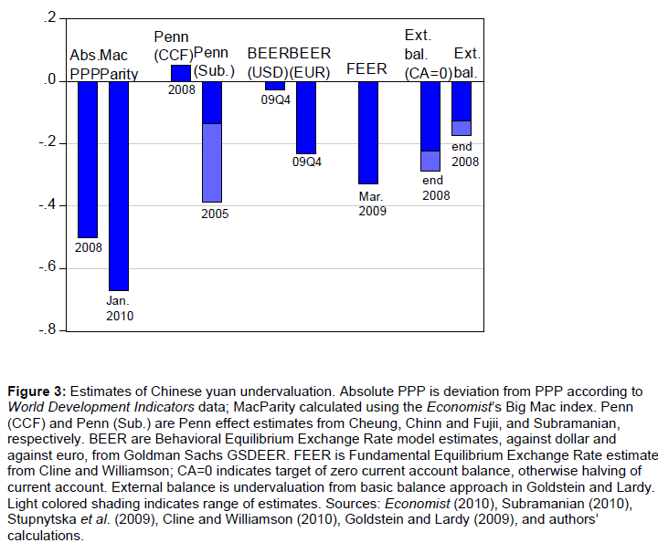
I summarize the typology of studies in this table (which is adapted from Cheung et al. (2006).

Given the variety of concepts, multiplied by the number of statistical methodologies, and data sources, it’s no wonder estimates of misalignment differ. Figure 3 from Cheung, Chinn and Fujii (in Evenett (ed.), US-Sino Currency Debate, 2010) highlights the wide variation in estimates in the latter part of the 2000’s.

For everything one wants to know about purchasing power parity and real exchange rates determination, see this recent survey.