Yes, exchange rate prediction once again. Last Thursday, Michael Moore (of Queen’s University Belfast) and I presented a new paper at the IMF’s conference on International Macro-Finance (co-sponsored with the ESRC funded World Economy and Finance Program). Here’s the paper [pdf].
In this paper, we introduce a novel data set, namely foreign exchange order flow spanning a eight year period. This far exceeds other order flow data sets, and allows us to investigate in a more comprehensive and innovative fashion the added explanatory power of order flow over conventional monetary model fundamentals — namely the money supply, income levels (as proxied by GDP), short term interest rates and inflation rates.
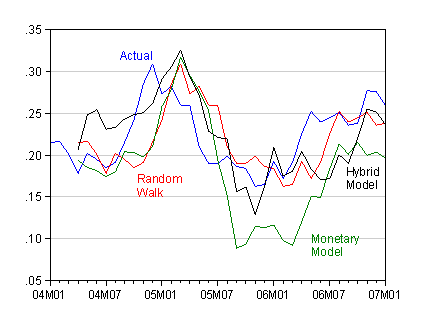
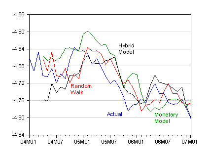
In order to anticipate the results, we find that incorporating order flow into the typical monetary model specification leads to plausible parameter values for the long run relationship. Furthermore, in out-of-sample forecasting exercises (formally, ex post simulations) the hybrid specification incorporating order flow outperforms the monetary model at horizons up to six months for the USD/EUR and the USD/JPY. In addition, the hybrid model outperforms a random walk most of the times.
First, a recap as to the challenge that faces us. In this post from several months back, I laid out the difficulties that conventional macro models of exchange rates face. While it is relatively easy to find “good-fitting” equations, the estimated equations rarely perform well in out of sample forecasting exercises. In such procedures, a regression is estimated over a given sample period, and then this relationship is used to forecast out several periods, using the actually realized values of the right hand side variables. The resulting forecast error is then recorded. The estimation sample is then moved up one period, and the procedure repeated, until all the observations in the period reserved for out-of-sample forecasting are exhausted. Note that this is not a true forecasting exercise which would be useful for trying to exploit profit opportunities. Rather it is a form of robustness check, to determine whether the overfitting of the data has led to inappropriate statistical inferences. Generally, estimated models perform badly, relative to a random walk, in such exercises. For a recent survey, see Cheung, Chinn and Garcia-Pascual (2003).
In that post, I noted one explanation forwarded by Frydman and Goldberg [1], was that imperfect knowledge expectations was a better characterization than rational expectations.
In our paper,we take a different tack. We motivate our analysis by arguing that the conventional monetary model encounters empirical difficulties because it assumes stability of the money demand equation (or for the monetarists in the audience, random velocity shocks). While it is simple in principle to allow for such shocks to preferences that would manifest in velocity changes, empirical counterparts to such shocks are hard to identify. We take order flow as representing shocks to those preferences.
This results in a specification implying a long run relationship between the exchange rate, the conventional monetary fundamentals, and cumulated order flow. In econometric terms, there should be a cointegrating relationship. We use the Johansen maximum likelihood approach to determine whether a cointegrating relationship exists. On the basis of the finite sample critical values (Cheung and Lai, 1993), we determine that there exists ample evidence for at least one such cointegrating relationship (multiple ones are not ruled out).
We estimate a set of error correction models.
dxt = f(dmt-1, dyt-1, dit-1, dpit-1, oft, ectt-1)
Where ect is the “error correction term”, that is the deviation from the long run cointegrating relationship, as identified using dynamic OLS; m is the inter-country (log) money differential, y is the income differential, i is the interest rate differential, pi is the inflation differential, of is order flow, and d is the first difference operator. We find that (1) contemporaneous order flow almost always enters in as a statistically significant variable, and (2) cumulated order flow enters into the long run relationship significantly. Order flow enters in these cases with the correct sign.
What about out of sample forecasting (recalling that these are tests for robustness)? We find that the hybrid model, incorporating order flow, outperforms a monetary model in almost all instances, according to a RMSE criterion. In addition, the hybrid model always outperforms the Evans and Lyons specification (incorporating interest rates and order flow) for the USD/EUR.

Figure 1: Log USD/EUR exchange rate (blue) and forecasts from random walk (red) Monetary (green), Hybrid (black). Source: Chinn and Moore (2008).

Figure 1: Log USD/JPY exchange rate (blue) and forecasts from random walk (red) Monetary (green), Hybrid (black). Source: Chinn and Moore (2008).
From this we take the finding that the monetary model should not be dispensed with. Money fundamentals do matter; what is necessary is for some proxy measure to enable one to accommodate empirically velocity shocks. Once that is accomplished, the monetary model appears much more empirically valid than it otherwise seems.
Technorati Tags: exchange rate,
monetary model,
order flow intervention, velocity,
interest rates.
Sounds like a fascinating paper (I’m looking forward to reading it.) The order flow data also sounds like an important contribution by itself.
One question that’s been bothering me about the monetary model of exchange rates, however, is the data revision problem. As Amato and Swanson have pointed out, monetary aggregates undergo substantial revisions ex post. In their study, the revisions are so severe that while the revised data have explanatory power, the series originally available to forecasters do not.
Of course, some researchers say this does not matter; the most recent series are our “best” measure and capture whatever the “fundamental” economic forces were at the time, whether agents were aware of it or not. However, it makes me wonder about nature of our standard “out-of-sample” forecasting experiments. Do we know whether the our measures of money were revised ex post to explain better the movements of exchange rates? Or are the revisions uncorrelated with subsequent exchange rate movements?
I am a little puzzled – does this specification still beg the question of what ultimately drives order flow/velocity shocks?
For example, is it asset managers becoming net sellers/buyers of assets denominated in a currency?
SvN: Interesting point. For us, we are concerned mostly about the issue of whether macro fundamentals “explain” movements in exchange rates, rather than in a true forecasting sense. Obviously, those two are related, but I view them as having different implications for predictability using the final revised data.
By the way, regarding the use of real-time vs. final-revised data, in exchange rate determination, you should see Jon Faust, John Rogers, and Jonathan H. Wright, “Exchange Rate Forecasting: The Errors We’ve Really Made,” Journal of International Economics 60 (May 2003).
And did they outperform the random walk?
Read it, liked it, even put my real e mail address in the post.
Each new innovative revelation causes a series of updates to the buyers “inventory management”. The update rate is limited by the transaction rate.
Barkley Rosser: No. Excellent paper, nonetheless, for other reasons.
Menzie:
Does the type of monetary aggregate used in the analysis affect the results? Similarly, would there be any gains to this exercise if one could determine the proper measure of money?
David: In-sample fit, M2 vs. M1 does not matter. Have not tried Divisia. My impression/vague recollection is that use of Divisia indices do not change the performance of estimated monetary models along either in-sample or out-of-sample dimensions.