Today we are fortunate to present a guest contribution written by Ali Alichi, senior economist at the International Monetary Fund. The views expressed in this blog are solely those of the author and do not necessarily represent the views of the IMF, its management, nor its Executive Board.
Models with deterministic trends, such as the HP filter or the “hybrid” approach of the Congressional Budget Office (CBO) produce unreliable estimates for the potential output. For example, excess capacity built in the run-up to the Global Financial Crisis (GFC) should be treated as cyclical, but deterministic-trend models initially treat it as permanent, leading to an overestimation of potential output and a large output gap in the aftermath of the Crisis. In a recent paper, we have developed a multivariate (MV) filtering methodology, which tackles this issue for the U.S. economy, among other desirable features.
Methodology
The MV filtering methodology extracts the unobservable potential output from observables (output, employment indicators, capacity utilization, inflation indicators, etc). This is done by (i) breaking all variables into structural and cyclical (shock) components, (ii) writing down the economic relationship between variables, e,g,, the Phillips curve, which connects output to inflation, and (iii) estimating the whole system using the data for observables and economic relationships for unobservables. In particular, estimates draw on labor market data, capacity utilization, inflation, and inflation expectations. Not all of this data and economic relationships usually enter traditional estimates, making it hard for them to identify which shocks have longer lasting effects on potential.
Findings
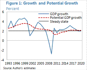
Potential growth has gradually recovered toward 2 percent after the GFC. Figure 1 shows the paths of (real) GDP and potential GDP growth.1 In the second half of 1990s, potential growth reached about 3½ percent, but since early 2000s, it started falling. The GFC brought activity to a halt and potential output growth to the negative territory. Potential growth started to pick up in 2010, and is currently estimated at around its steady state growth rate of about 2.0 percent. Potential growth is expected to surpass its steady state value in the next 2-3 years, as the recovery picks up steam but will slow down to its steady state value of 2.0 percent as demographic effects set in.
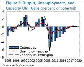
The U.S. output gap has shrunk considerably since the GFC, but is still negative. The U.S. output gap reached about -5¼ percent, following the GFC, but has since been recovering. By end-2014, the output gap stood at around -2.0 percent. It is projected that the output gap would continue shrinking and would be closed in 2017.
Comparing the MV filter results with other estimates
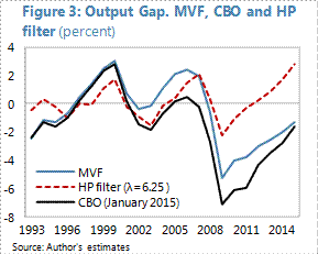
Traditional methods do not capture legacy effects properly. Figure 3 shows a comparison of output gap estimate for the MV filter, CBO, and HP filter. For 2014, the MV filter’s and CBO’s extimates are very close to each other. However, the paths of these two series before are markedly different, with the CBO projecting a noticeably larger output gap after the GFC than the MV filter. This is because the MV filter interprets some of the capacity that was built in the runup to the crisis as a temporary shock. CBO’s methodlogy, howver, initally treats most of the capacity built in the run up to the crisis as permanent, given its deterministic-trend approach. This changes over years as weak data on growth inform CBO’s projections that a sizable part of the capacity built before the ciris was not permanent, brining CBO’s estimate closer to MV filter’s estimate over time, in the absence of additional crisis. Figure 3 also reports the results of an HP filter with the actual growth data up to 2014. In the next section we show that HP filter’s estimates vary significantly as more data is available, making it very unrelibale to estimate the potential output and output gap.
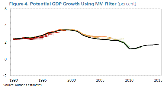
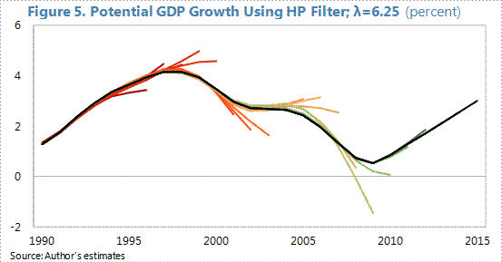
Tackling the end-of-sample problem
A well known problem with filters, such as the HP, is the end-of-sample problem. As data is added to the end of the sample, projections change significantly. MV filters are also generally subject to this end-of-sample problem. The MV filter resolves this issue by drawing on information from growth and inflation expectations. Figures 3 shows estimates of output gap, using our MV filter, as well as the HP filter. Estimates of potentail output for the MV filter are presented in Figure 4, and for the HP filter are presented in Figure 5. In Figures 4-5, potential output is projected for 5 periods ahead and with each additional year, the sample is extended by one year and potential output is reestimated. Out-of-sample estimates from the MV filter remain much closer to the final (current) estimate, which is shown in black, while for the HP filter, out-of-sample estimates substantially deviate from the final (current) estimate. This is largely because the MV filter uses the information in growth and inflation expectations to inform its projections, but the HP filter does not.
Conclusion
So, have the scars from the GFC healed? Not yet. The output gap is still negative and potential has yet to recover to its new long-term level. But irrespective of what methodology is used, there is a consensus that the output gap is shrinking.
This post written by Ali Alichi.
1. In Figure 1, real GDP growth until 2014 is from actual data from the Bureau of Economic Analysis, but for 2015 and onwards, it is MV filtering model’s projection. Potential GDP growth is model’s estimate\projection for the entire sample.
It’s an amazing conclusion. The output gap will close after two more years of depression.
Ali, do yiu have any comments on secular stagnation? Because I take from this that the whole sec-stag debate was a waste of time. It was just a typical boom and bust cycle, and soon enough we will return to our long term trend….
Empirically, we have some “financial crisis” about every 10 years, and every 40 years a serious one, roughly.
The US at that point in 2018 just stabilizising the overall system, at a 110% peace time debt, when the next SHTF, like 25% overvalued houses (my Case Shiller data analysis) crashing, the 20% overvalued (hyper simplified , e.g. look at pe ratios of SPY vs EWG) american stock market crashing.
Spice this scenario up a little with China crashing, going belligerent, and a chinese sub colliding with, and sinking a US carrier in the South China Sea.
By how much would American demand fall ? 6% 8% 10% ?
Inflating away will not work this time,
please look at http://de.slideshare.net/genauer/sampler-2-of-imf-2014-weo-data-plots page 8 and 9 for real long term (300 years) data and how the US&UK inflation strategy worked in the 1970ties.
But even before the great recession there was significant evidence that long term growth had already slowed.
So what is potential output still looks like an unresolved issue even if this approach is proven superior.
I’m more interested in what is the long run growth of productivity. If we can get that right, estimating potential output is easy.
Long-term growth didn’t slow much, until 2008, even with rising oil prices and larger trade deficits throughout the 2000s.
Then the downshift, in growth, was sudden, severe, and, since 2009, sustained. Chart:
http://www.advisorperspectives.com/dshort/charts/indicators/GDP-per-capita-overview.html?GDP-per-capita-since-1960-with-regression.gif
It was falling beforehand, don’t even try to say otherwise. It didn’t start falling to new lows until 2010 when the labor force contracted in new entrants. The facts are facts. The US grew to much between 1996-2006 and the correction was obviously made. Real housing demand actually peaked in the mid-90’s, when no surprise, was when the Baby Boom demographic top peak hit in terms of labor market entrants.
It was slowing, remaining above the trend line, but didn’t fall, till after the peak in December 2007.
It was a mild recession, till Lehman failed in September 2008.
The trough was in June 2009, although unemployment is a lagging indicator.
And, there was about twice as many new houses sold in the mid-2000s than the mid-1990s. Chart:
https://research.stlouisfed.org/fred2/series/HSN1F
You should be interested in productivity at full employment.
There are too many idle inputs or hours. So, output is too low.
You might want to read the latest from me.
VMT and GDP.
http://www.prienga.com/blog/2015/7/21/uk-vmt-its-also-recovering
Technical question on Fig 4. The model parameters were determined using the full data set and then only given the data up through year X and asked to forecast years X+1 through X+5? Or the model parameters were re-derived using only data up through year X? I ask because the forecasts look almost too good; in 2005, a sharp downturn in potential GDP growth was forecast to occur in 2010? Really? It looks to me like the model may have been overfit, with too many parameters relative to the length of the data.
Question for Mr. Ali Alichi,
Why did you compare your method to CBO forecasts of potential GDP rather than Federal Reserve estimated? My understanding is that the use of H-P filters is more in the spirit of the Federal Reserve’s approach. CBO says that they use a Solow model approach.
It is difficult to envision potential GDP growth doing anything but declining on trend from now on. Numerous impediments have arisen in recent years that spell ongoing decline. More on the impediments below. First, PeakTrader points to a chart of per capital real growth with a linear trendline that’s not as meaningful as first appears.
The trendline of average growth since the 60s may hide more than it reveals. Instead look at a tangent line laid atop cycle peaks. The slope of this tangent will be only slightly different from that of the trendline on the chart. This tangent line touches each cycle peak from the pre-1974 peak to the pre-2001 peak. This different way of looking at things, then, delineates 3 segments of per capita GDP growth: rapid growth early on, medium growth ’73 to ’00, and slow growth since. This can be further refined. The odd decade is the 90s. It interrupted a trend already underway. The growth spurt in the second half of that decade was an anomaly. This spurt is widely attributed to a short-lived technology boom. The Pentium chip and Windows 95 were the innovations. But this is not the whole story. Also, Y2K fears drove an investment boom. Together, equipment and intellectual capital investment contributed 0.6 ppts to real GDP growth the 5 years through 1995:2, picked up to 1.1 ppts the next 5 years, then fell abruptly to 0.2 ppts the following 5 years. Some of the late-90s growth simply stole from the future.
The secular decline set in in earnest after the 60s. That this decline is permanent will become more and more apparent. I do not mean permanent in the strict sense of the word. But a realistic assessment of the political and cultural spheres which interact with the economic sphere make permanent decline very likely. Impediments to growth have set in, each at various points along the way. Most prominent are: the burden of debt, the trade deficit, size of government, regulatory burden, shortfall of national saving that translates into poor net capital formation, and most recently an unparalleled interference with market pricing by ZIRP and QE. Educational attainment (as measured by international scores) and work ethic are also in secular decline. The latter affect the most important resource of all: human know-how. For the bulk of the workforce, most know-how comes about through experience on the job. And it has a high decay rate.
Evidently given its newest projections of less than 2% potential going forward, the Fed is coming around to this view too. As the West declines relative to the East in share of global GDP – the relative share widening in favor of the East at a rate of about 1½% annually! – the odds of a major war will rise exponentially. At some point sooner than might be expected, the US dollar will lose reserve currency status. As well, greater complexity and the historic global debt burden increase the likelihood of more, and more severe, financial crises ahead. Secular stagnation is not a bad name for this. All that’s left is to add the adjective accelerating.
“Models with deterministic trends, such as the HP filter”
wrong! HP filter has a stochastic trend
When you look at what drove productivity historically,
you can discern 3 distinctive factors:
a) people moving off the farm to all-year industrial work (roughly a factor of 2)
Now Farmers are less than 1% of the population in western countries. There is no further optimization at that point. All those small steaders generously subsidizd in Europe in the 1960s – 1990ties are retired by now.
b) people getting longer and better education
That was a boost of some 2 x 2 for primary and secondary education. That factor has in most places saturated as well. 12 years of school, the number of people attending university does not rise in the US. Germany says 9 years school plus 3 years apprenticeship is actually better. some 25 -30% attending university.
There is no point in educating people with stuff , half of it they forget over the summer. Why teach people the law of gravity, if none but the physics degrees remember it 10 years later? (I checked this personally with a sample of by now sufficient size : – )
Here in Germany we wonder what good 50% tertiary education is in places , which do not have substantial manfuacturing (https://en.wikipedia.org/wiki/List_of_countries_by_25%E2%80%9334_year_olds_having_a_tertiary_education_degree)
How many sociologists or english majors can be employed productively, where and how? With having substantial tech manufacturing, Germany somehow manages with just 27% “tertiary”. Why is that so ? Ever thought about? By switching to the Anglo Bachelor / Master system we effectively cut the university years for half of them by 3 years, compared to the former “Diplom” system with average study time of 6 or more years
c) Getting the women into the regular workforce
About a factor of 1.6. That has sizzled out by now in most places as well. Even in catholic Bavaria they now have to bow to the constitutional court declaring Betreuungsgeld not legal : – )
To look at it from a somewhat different angle:
A) Productivity gains in agriculture do not translate to society anymore, because the 1% fraction is way too small
B) Productivity gains in manufacturing do not translate anymore, because it just leads globally to reduction of the related workforce
(in 1990 the manufacturing percentage in my German birth town was still over 50%, now it is below 20%, in most US places the process has been more gradual)
C) with about 80% of the population in “Services”, because not needed in Agriculture, mining, industry, most of those jobs “do not scale”, have limited to none productivity improvement potential:
Cleaning ladies, nurses, lawyers, hair cutters, sales girl, plumber ….
That leaves us to the historical “technical” productivty gains of 0.5 – 1% per anno, when excluding the tapped out 3 factors above, and even this is difficult to achieve
It’s amazing what people can conclude without considering first the replacement of the lost demand.
gosh , the US government was substituting private “demand” to the tune of 12 % government deficit in 2009, in peace times !
IMF April 2015 WEO data for US givernment deficit in % GDP
from 2008 on:
-4.961 -11.58 -9.23 -7.62 -6.327 -3.62 -3.223 -2.172
and, are you better off than Germany? which had to finance the rebuilt of Eastern Germany, at a cost of about 100% of Western GDP