While Wisconsin lags, and statistically significantly so…
From CEA Chair Jason Furman:
The economy added 215,000 jobs in July, while the unemployment rate held steady at 5.3 percent—its lowest level since 2008. Over the past two years, our economy created 5.7 million jobs, the strongest two-year job growth since 2000. And our businesses have created 13.0 million jobs over the past 65 straight months, extending the longest streak on record.
Figure 1 shows private nonfarm payroll employment in the US and Wisconsin, normalized (in logs) to 2011M01=0.
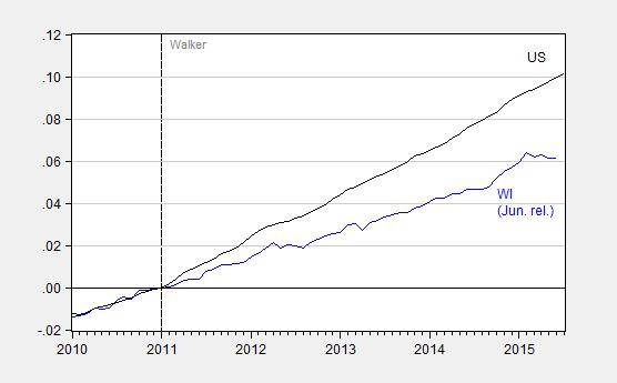
Figure 1: Log private nonfarm payroll employment in US (black) and Wisconsin (blue), both normalized to 2011M01=0. Source: BLS and author’s calculations.
Since the beginning of Governor Walker’s first administration, cumulative private employment growth has lagged the Nation’s by 3.9% (log terms).
Since Wisconsin’s trend employment does not necessarily match the Nation’s, it makes sense to ask what one should have expected Wisconsin’s employment growth to be, given historical correlations. One way to do this is to estimate the relationship between US and Wisconsin employment through 2010, then use this relationship to forecast dynamically out-of-sample Wisconsin employment through 2015M07 using ex post realizations of US employment.
Here is how I implemented this procedure.
1. I used the maximum sample period available for in-sample estimation, while allowing for sufficient lags, i.e., 1990M06-2010M12.
2. Test for stationarity of log US and WI private NFP. I fail to reject I(1) processes.
3. I test for cointegration, using the Johansen maximum likelihood approach, allowing for trend in VAR, constant in cointegrating equation. The no cointegration null is rejected at the 5% msl using asymptotic critical values, according to the trace and maximal eigenvalue statistics.
4. I then estimated a single-equation (unconstrainted) error correction model over the 1990M06-2010M12 period.
5. The estimated equation is then used to conduct a dynamic out-of-sample forecast.
The estimated equation is:
(1) Δnt = -0.0014 – 0.041×nt-1 + 0.028×nUSt-1 + three lags of first differences + ut
Adj-R2 = 0.47, SER = 0.0018, DW = 2.00, Obs.=216247, sample 1990M06-2010M12. Bold face denotes significance at the 10% MSL, using HAC robust standard errors.
Using the DW statistic is not valid for assessing the presence of serial correlation when there’s a lagged dependent variable in the regression, but Q(12) and Q(24) tests fail to reject the no-serial correlation null.
The implied long run elasticity of Wisconsin to US private NFP is 0.69; using the Johansen procedure (no trend in cointegrating vector, four first difference lags) yields a long run elasticity of 0.73, while DOLS(+2,-2) yields an estimate of 0.80. The maximum likelihood and DOLS estimates indicate one can reject the null that the elasticity is unitary.
Figure 2 presents the resulting dynamic out-of-sample forecast, along with the 90% forecast interval.
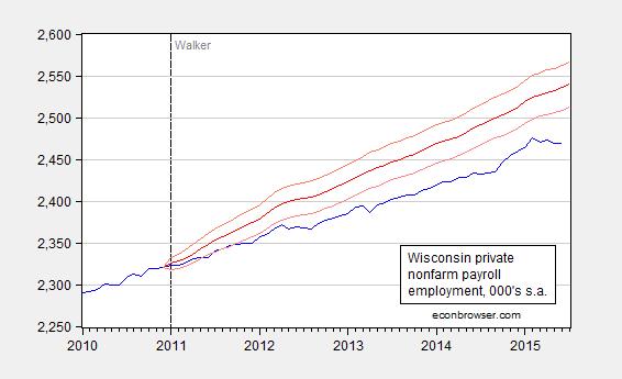
Figure 2: Wisconsin private nonfarm payroll employment, June release (blue), and out-of-sample forecast (red), in 000’s, s.a. 90% forecast interval (pink). Source: BLS and author’s calculations. See text.
The results indicate that Wisconsin private employment has been lagging what one would have expected given historical correlations with US employment.
Regression output is here. The methodology roughly follows that in Chinn (JPAM, 1991) (paper is sans Johansen and Juselius).
Update, 8/10 1pm Pacific: Here for completeness is a graph of Wisconsin employment trends (downward) according to establishment and household surveys.
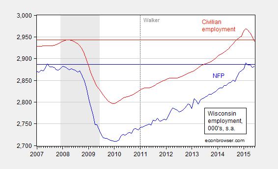
Figure 3: Wisconsin nonfarm payroll employment (blue) and civilian employment (red), and corresponding peak levels (dark blue, dark red). NBER defined recession dates shaded gray. Source: BLS (June release), and NBER.
Professor Chinn,
I come close to your output, but not exact. My output is: -0.011 – 0.042xn(t-1) +0.029xnus(t-1). Adj Rsqd=0.47, SER=0.0019, DW=2.00. My output says 243 observations after adjustments. My 2016 dynamic forecast amount for Wisconsin at 2015m06=2,530,146.
Any chance of posting your output and cointegration test as you graciously did for your “A Parsimonious Error Correction Model of Kansas Economic Activity”,6-2-15?
Thanks
AS: I typed the wrong NObs; it’s 247. I have posted the regression output at the end of the post, and here.
I added the Kansas output a while ago, under the equation. Here is a direct link.
Professor Chinn,
Thanks! As mentioned in the past, I appreciate learning from you. I had copied the Kansas output back in June. Thanks for additional link.
Unfortunately, I don’t understand why my model adjusts the 247 sample observations to an adjusted sample of 243. My adjusted sample includes 1990m10 to 2010m12, even though input sample includes 1990m06 to 2010m12.
AS: I think you restricted the sample to 2000M06-2010M12, and then generated the difference variables. I suggest you use the whole sample, generate the difference variables, then restrict.
Professor Chinn,
Thanks.
My number of observations now shows as 247. The output is close, but not exact. Your C =-0.008406 vs. mine=-0.008966. Your first coefficient = -0.041080 vs. mine = -0.041393. Your second coefficient =0.028213 vs. mine=0.028471. Your adj. Rsqd=0.473058 vs. mine=0.473235. Your SER=0.001844 vs. mine = 0.001844.
Professor Chinn,
The P-value on the -0.041080 coefficient is 0.0047, and the P-value on the 0.028213 coefficient is 0.0222. Why do you say the coefficients are significant at the 10% MSL, using HAC robust standard errors? Why am I wrong thinking the significance level is 5% MSL?
AS: You are not wrong. Those coefficients are significant at the 5% msl as well (and at the 1% for the former), but I didn’t want to try to denote all those different significance levels with astersisks, etc. So, I adopted a short-hand for reporting the equations in the post, which I wouldn’t do in a formal academic paper.
Thanks! I understand your reasoning for the short-hand reporting. Just wanted to make sure I was not off in the woods somewhere.
AS: I applaud your diligence. I once again recommend Enders, Applied Econometric Time Series (Wiley) for a practical example-laden approach, and Hamilton, Time Series Analysis (Princeton) generally.
Menzie’s UW colleague Noah Williams provides a different analysis here;
http://www.ssc.wisc.edu/~nwilliam/wisconsin-economy.htm
‘ The unemployment rate in Wisconsin did not spike as dramatically as in the rest of the nation during the recession, but even from the lower peak it has fallen rapidly, especially over the past couple of years. Since the beginning of 2014 the unemployment rate has fallen by 1.5 percentage points, and now stands at 4.6% in comparison to the 5.5% national average.
‘In addition, a significant component of the reduction in the unemployment rate nationwide has been a decline in the labor force participation rate. Some of the decline in participation has been due to longer run demographic factors, driven by the aging of the population. However a significant component has been a cyclical, with unemployed workers stopping searching for a job. The labor force participation rate in Wisconsin has historically been above the national average, and it has declined since 2007, but it has increased over the past year and has been roughly stable since the beginning of 2012. By comparison, if the labor force participation rate in the US as a whole had remained constant since January 2012 (rather than falling by one percentage point), the national unemployment rate would now be 7.0% rather than 5.5%. Thus the national unemployment rate hides some additional weaknesses in the labor market which are not present in Wisconsin, as participation in the state has remained strong and even increased as the unemployment rate has fallen.’
Patrick R. Sullivan: This post along with this post on median incomes addresses the points Noah brings up.
I am still waiting, now nearly a year later, to hear you admit you were in error regarding depth of the downturn in Canada vs. US during the Great Depression. As you recall, you stated unequivocally:
And this statement is wrong.
Patrick R. Sullivan: Please also consult this post. Both Wisconsin employment series — including civilian employment that incorporates farm employment — are below pre-recession peaks.