The dramatic decline in the prices of a number of commodities over the last 16 months must have a common factor. One variable that seems to be quite important is the exchange rate.
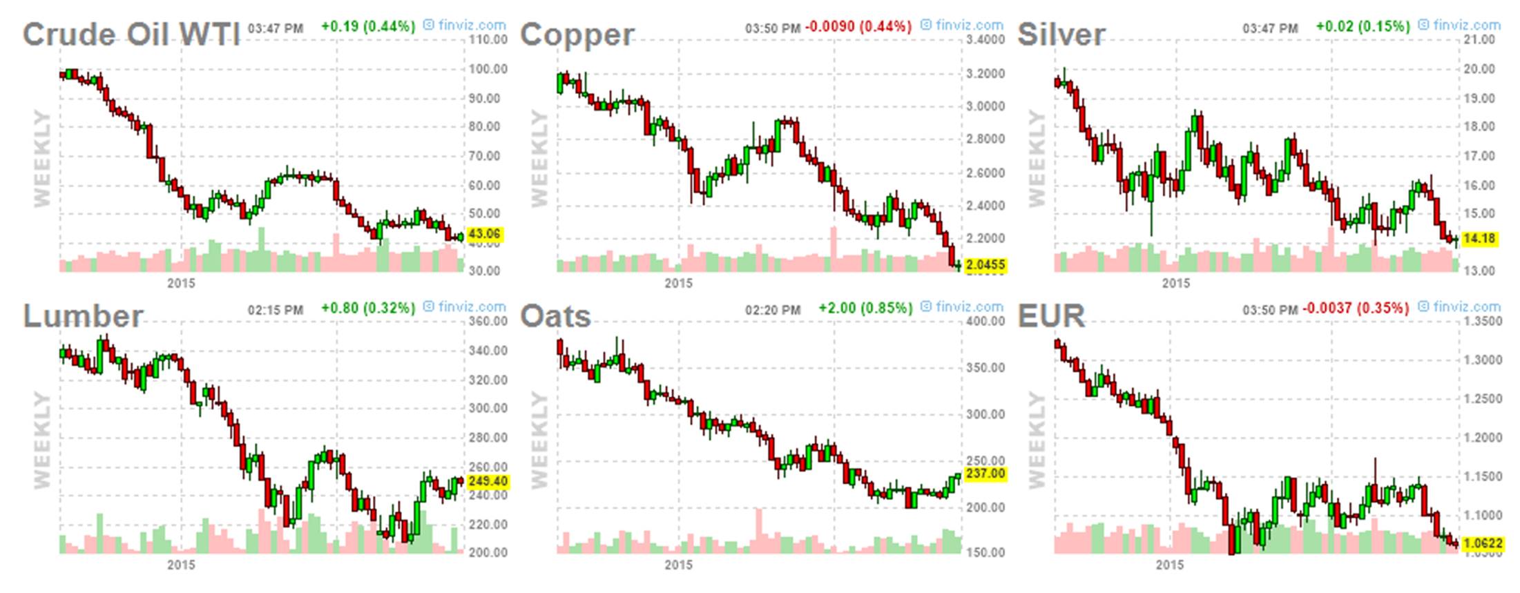
Dollar prices of five commodities along with dollar cost of one euro. Source: Financial Visualizations.
Here’s a graph over a longer period of the dollar price of oil, the dollar price of copper, and the dollar price of a weighted average of other countries’ currencies with weights based on the volume of trade between the U.S. and each country. The graph is plotted on a logarithmic basis, so for small changes the height of each series corresponds to the percent difference between the price at the indicated date and the price at the end of June 2014 (see my primer on the use of logarithms in economics if you’re curious about those statements or why it might be helpful to plot series this way). The plunge down in all three measures since June 2014 that was highlighted in the first set of graphs is seen to be a broader pattern of striking positive co-movements among these variables.
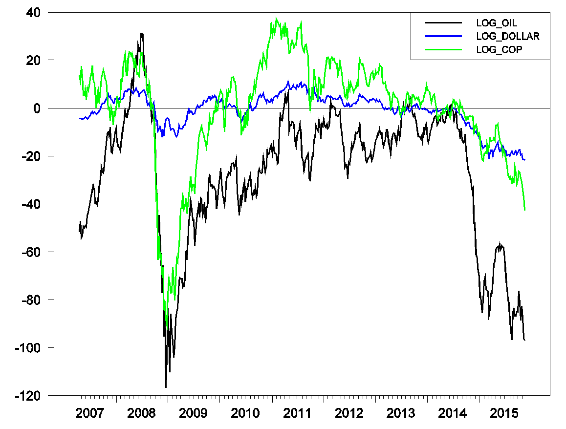
Price of West Texas Intermediate (black), copper (green), and inverse of trade-weighted value of the dollar (blue), end of week values April 20, 2007 to November 20, 2015. Graph plots 100 times the difference between the natural logarithm at the indicated date and the natural logarithm on June 27, 2014. A value for the blue series below zero means that the dollar was worth more on that date than it had been on June 27, 2014.
One would expect that when the dollar price of other countries’ currencies falls, so would the dollar price of internationally traded commodities. But it is a mistake to say that the exchange rate is the cause of the change in commodity prices. The reason is that exchange rates and commodity prices are jointly determined as the outcome of other forces. Depending on what those other forces are, one might see stronger or weaker co-movement between commodity prices and exchange rates.
For example, the most striking episode in the graph above is the Great Recession in 2008-2009. Falling GDP around the world meant falling demand for commodities. It was also associated with a flight to safety in capital markets, which showed up as a surge in the value of the dollar. It’s not the case that the strong dollar then was the cause of falling dollar prices of oil and copper. Instead, the Great Recession was itself the common cause behind movements in all three variables.
One way to get a sense of how the driving factors have changed over time is to look at a regression of the weekly logarithmic change (approximately the weekly percentage change) of the dollar price of oil on the weekly logarithmic change in the exchange rate using a rolling 2-year window. Each point in the graph below plots that estimated coefficient using a sample of two years’ data ending at the indicated date. The coefficient was above two during and after the Great Recession– if the dollar appreciated 1% during the week in that period, you would expect to see more than a 2% decline in oil prices. The coefficient fell below one in the first half of 2014 but has since risen back above one.

I had been giving a similar interpretation to the correlation since June 2014 as to the data from the Great Recession– news about weakness in the world economy seemed to be a key reason for strength of the dollar over the last year and a half, and would also be a reason for declining commodity prices.
However, developments of the last three weeks call for a different explanation. The October 28 FOMC statement and subsequent statements by Fed officials have made clear that a hike in U.S. interest rates is coming December 16. An increase in U.S. interest rates relative to our trading partners is the primary reason that the dollar appreciated 4% (logarithmically) since October 16. Over that same period the dollar price of oil and copper each fell 16%.
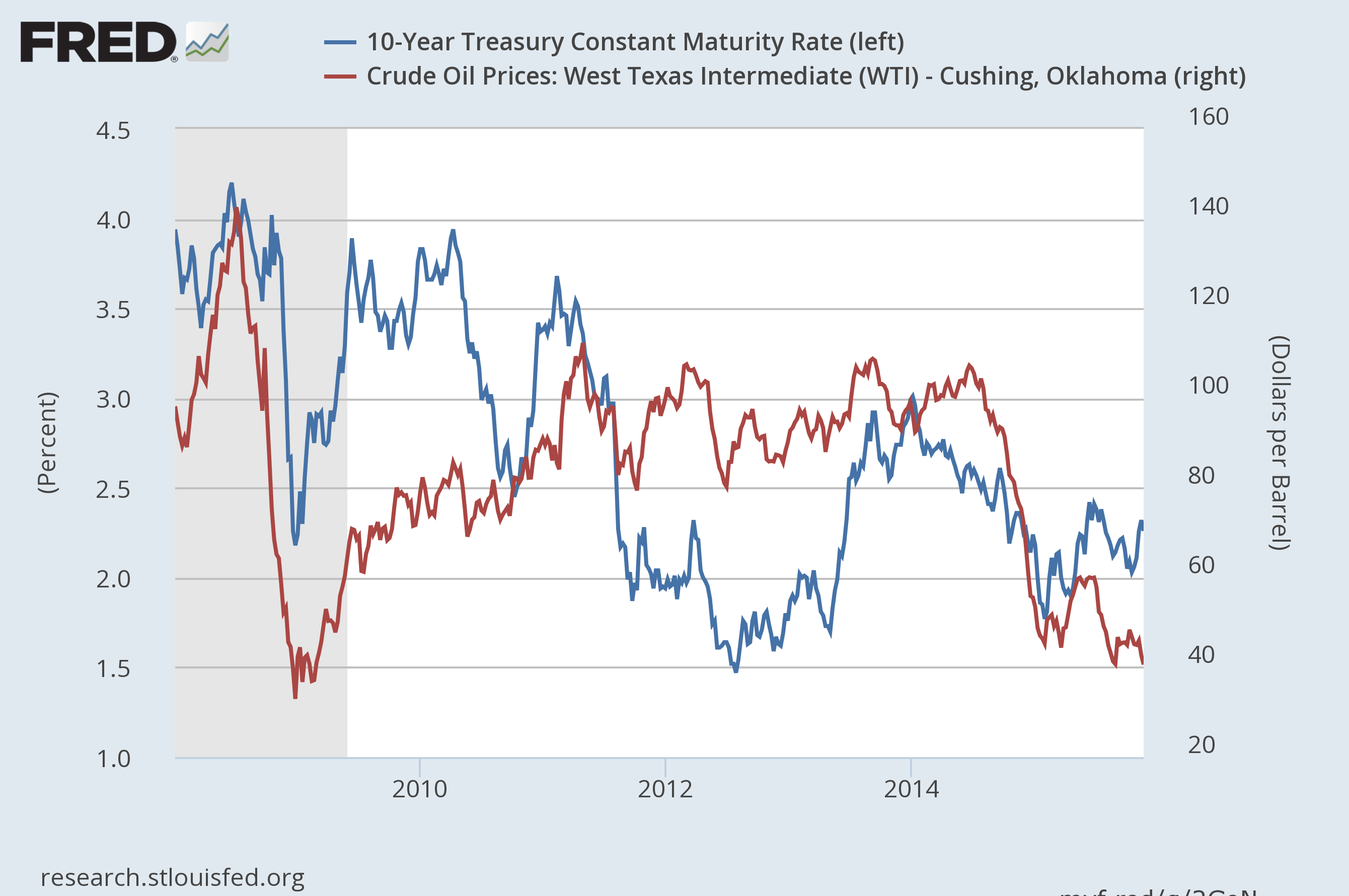
Jeff Frankel has long suggested that higher interest rates lead directly to lower commodity prices through a variety of channels. For example, if the Fed raises interest rates, that may reduce the level of economic activity and thereby lower commodity demand. But the recent correlation is in the opposite direction. Over the past 5 years, if long-term interest rates fall, oil prices likely do as well. My interpretation of this pattern has been that falling interest rates are a response to a weaker global economy, which itself is also a contributing factor to lower oil prices.
For some time I’ve been using a simple summary of these various correlations in the form of a regression of the weekly change in the price of oil on that week’s change in the price of copper, the value of the dollar, and the interest rate on a 10-year U.S. Treasury bond. The regression is estimated over the period from April 2007 to June 2014. The price of oil was more likely to decrease in a given week if the copper price also decreased, the dollar appreciated, or interest rates fell. The overall decline in copper prices, appreciation of the dollar, and decline in interest rates since June 2014 would have led one to predict that the price of oil would have fallen from $105/barrel in June 2014 to around $65 today, or about 60% of the observed decline. The actual and predicted price of oil that comes out of these calculations is plotted for each week since June 2014 in the graph below.
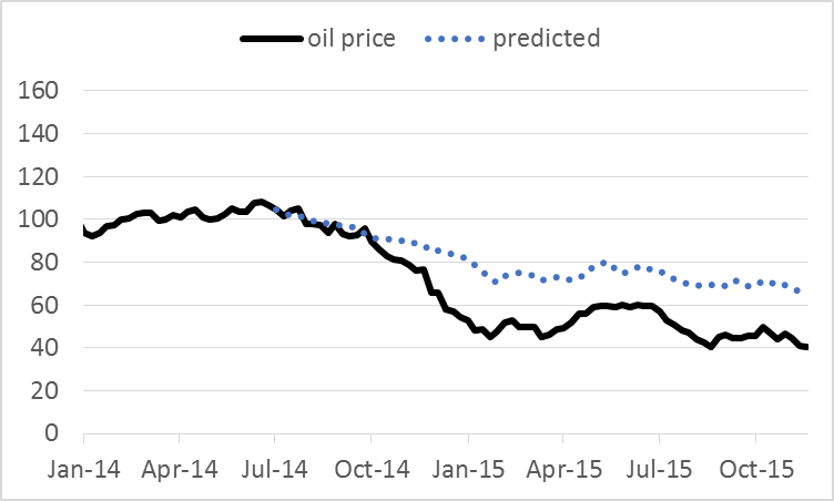
We have a friendly tool with data links that you can use to perform these calculations yourself for any start and end date of interest. For example, the model predicts that oil prices would have fallen from $47.30 on October 16 to $43.19 today, about half the observed decline. If all that had changed over that period had been the rise in interest rates, we would have expected to see the price of oil increase, not decline, over the last month. The observed decline in copper prices and appreciation of the dollar are more than enough to counteract that effect and account for a significant part of the observed decline.
Whether that’s a fully rational market adjustment is a question for which only time will give the answer. But I will offer the view, based on the market reaction so far, that if the Fed’s objective in raising rates is to lower U.S. inflation and GDP, it seems to have taken a significant step in that direction.
Perhaps, the market reaction is the expectation of stronger U.S. growth.
And, the market tends to overreact.
A Federal Funds Rate of 0.25% is still highly accommodative.
I think, in the end, the result on U.S. growth is uncertain or small.
https://research.stlouisfed.org/fred2/graph/fredgraph.png?g=2Kqp
https://research.stlouisfed.org/fred2/graph/fredgraph.png?g=2K3Z
https://research.stlouisfed.org/fred2/graph/fredgraph.png?g=2Kqr
https://research.stlouisfed.org/fred2/graph/fredgraph.png?g=2Kqv
https://research.stlouisfed.org/fred2/graph/fredgraph.png?g=2Kqs
https://research.stlouisfed.org/fred2/graph/fredgraph.png?g=2Kqw
Under the foregoing conditions, it is absolutely bizarre and surreal that the Fed would be determined to raise the reserve and discount rates PRECISELY NOW when they were cutting rates (with the exception of 1980) under similar conditions in the past.
Discount rate, funds rate, and reserves:
https://research.stlouisfed.org/fred2/graph/fredgraph.png?g=2KqA
https://research.stlouisfed.org/fred2/graph/fredgraph.png?g=2KqJ
https://research.stlouisfed.org/fred2/graph/fredgraph.png?g=2Kr8
https://research.stlouisfed.org/fred2/graph/fredgraph.png?g=2Krs
https://research.stlouisfed.org/fred2/graph/fredgraph.png?g=2Kr4
The Fed raised the discount rate in 1931 to support the US$ in response to the collapse of Creditanstalt and the devaluing of sterling by 25%, and again in 1933 to support the US$ prior to, or coincident with, FDR confiscating gold bullion and revaluing gold from $20.67 to $35 (devaluing the gold-exchange US$ by 40%).
https://www.frbatlanta.org/cenfis/publications/notesfromthevault/1001.aspx
http://www.federalreservehistory.org/Events/DetailView/27
After bank loans crashed 40-50% during 1929-33 and bank runs and closures occurred, excess reserves soared after 1933-34 (as has occurred since 2008) when bank deposits returned from coffee cans and mattresses following the creation of the FDIC.
The Fed increased reserve requirements in 1936-37 along with the US Treasury “sterilizing” gold inflows from Europe prior to the beginning of Hitler’s militarist expansionism.
Real private GDP:
https://research.stlouisfed.org/fred2/graph/fredgraph.png?g=2Krz
https://research.stlouisfed.org/fred2/graph/fredgraph.png?g=2KrI
US private real GDP per capita has averaged 0.5%/year since 2007 vs. real private GDP of 0% from 1929 to the late 1930s and again prior to WW II, and -0.06%/year per capita over the same period (US population in the 1930s to early 1940s was at a similar rate as today).
Japan’s private GDP and per capita:
https://research.stlouisfed.org/fred2/graph/fredgraph.png?g=2KrT
https://research.stlouisfed.org/fred2/graph/fredgraph.png?g=2Ks0
Adjusted for Japan’s population decline since the early 2000s, real private GDP per capita has averaged just 0.3%/year since the late 1990s.
http://tinyurl.com/p9e3yvz
Japan’s nominal GDP per capita is at the level of 1993-94.
For the progression of the Long Wave Trough to date, the US is aligning with the late 1930s and Japan in the early 2000s. The Fed and BOJ were cutting rates at that point.
https://research.stlouisfed.org/fred2/graph/fredgraph.png?g=2FRP
https://research.stlouisfed.org/fred2/graph/fredgraph.png?g=2FS6
With CPI at ~0%, the acceleration of TMS velocity to private GDP in a deep, recession-like, real, US$-adjusted contraction, the broad equity market in a bear market YoY, and nominal final sales less health care spending and the deficit decelerating well below the historical “stall speed” and recession threshold of 3% YoY, the Fed raising rates today is akin to the conditions in 1936-37.
Therefore, I expect that the Fed will be required in 2016 to maintain ZIRP, if not eventually NIRP, and resume QE to credit primary dealer banks’ balance sheets to finance the increasing fiscal deficit into 2017 or 2018 to prevent further deceleration or contraction of nominal GDP.
I suspect that by the end of 1Q 2016 the FOMC will be reversing course, and by the end of 2016 they’ll either have implemented or be actively considering negative interest rates.
“But I will offer the view, based on the market reaction so far, that if the Fed’s objective in raising rates is to lower U.S. inflation and GDP.”
More precisely, the Fed’s objective is to protect the elite by making sure that middle and lower class workers never get a wage increase.
What is surprising is that so many economists express bafflement at rising inequality.
“Stall speed”: https://app.box.com/s/0ulvltzk9w154gcs2zyoga3cshvg15ny
Again, under the current cyclical conditions, the Fed was cutting rates.
I notice you use the 10 year treasurer rate in your predictor. However, I understand that what might change in December is the Federal Funds Rate. It would seem to be useful to know what is the correlation between the two. In particular, absent some reverse QE, does the 10 year rate necessarily go up in lockstep?
Non-Economist: In the old days, if the fed funds rate went up 50 basis points, the 10-year rate might go up 25 basis points. The entire yield curve would shift up, but not one-for-one with the short end. The long rate would also go up in anticipation of a hike in the short rate– my view is that’s what we’re seeing here.
James:
Thank you. That is a reasonable answer to my question. But, does the bond market assume this is the good old days? Maybe, the FED is being swayed by nostalgia? In the current situation, can you tell by various economic indicators like personal income, etc. what is likely to happen to interest rates (at least for auto loans and mortgages) post December. I suppose if you could you would be rich.
Non-economist: The Fed has telegraphed pretty loudly and clearly what’s coming Dec 16. The main news to come is how long the Fed will take before implementing a subsequent change after that. I expect the Fed to be slow implementing the next step. So a good guess is that everything is already priced in to the yield curve, namely, that the movement we’ve already seen in the 10-year yield and the exchange rate is the effect what the of the next FOMC meeting is going to be. As I note above, the exchange rate effects are already pretty significant– I don’t see why the Fed would want to do much more any time soon.
Professor Hamilton,
As a learning question from an appreciative reader: While the analysis of the past is interesting, how useful is the analysis for future expectations when the past relationships seem to constantly change and the future price of copper, the future level of interest rates and exchange rates are currently unknown and perhaps difficult to forecast.
AS: You’re exactly right– I can’t forecast copper prices or the exchange rate. So this isn’t a forecasting relation. It’s a way of describing how different variables move together, which is important I claim for purposes of understanding the facts. As for instability, yes, the coefficients shift over time, but gradually.
The regression in the third graph uses a 2-year window, and the coefficient is always positive regardless of the window.
You can make a case that the most important “channel” that the 25 bp rate hike will be working through is actually the US dollar.
Appreciation in the US dollar quickly causes pressure on operating profits of American companies (the S&P 500 generates about 40%-45% of its operating income overseas), and reduces the competitive position of US exporters and by making imports cheaper, causes the US to potentially import deflationary pressures from overseas.
The FOMC is completely out-of-step with the inflation outlook in the US – we’re nowhere close to the 2% target for the PCE and haven’t been close to 2% since about 2011. Sheer madness, I believe.
We had a profits boom with weak GDP growth and we can have a profits recession with stronger GDP growth.
The oil glut, which is promoting U.S. consumption, will eventually end, putting downward pressure on the dollar.
And, if the labor markets strengthens, we may soon see wages rising faster.
Just because inflation is low now doesn’t mean it’ll be low in the future.
If you believe raising the Fed Funds Rate to 0.25%, at this point, is excessive, maybe you believe another round of QE is needed instead.
Just because we had profits boom with weak GDP growth absolutely doesn’t mean that we’ll have a profits recession with stronger GDP growth. What kind of logic is that?
We had profits boom with weak GDP growth because capacity utilization was very low after the last great recession, and because companies were so leveraged and weakened by the great recession that their first objective in the nascent recovery was to rebuild liquidity. After that, the recovery was weaker than a typical recovery and the level of uncertainty regarding tax policy and government policy and healthcare policy (especially) was very high, so with ample production capacity, why would companies rush to hire workers or expand plant and equipment? Against that backdrop, profit margins boomed and continued to boom. In past recoveries, we got a big capital spending cycle but not this time.
Real quarterly final sales measured year-over-year have been plugging along at the +2% level with a lot of consistency, and hardly seem poised for a breakout to the upside. Additionally, as much as the Fed might like to think they control the money supply, in the absence of lending growth the money supply doesn’t do anything – see the excellent Bank of England paper here:
http://www.bankofengland.co.uk/publications/Documents/quarterlybulletin/2014/qb14q1prereleasemoneycreation.pdf
which does an excellent job of explaining how “the majority of money in the modern economy is created by commercial banks making loans”.
In the absence of banks making loans (to creditworthy customers, I might add), money supply is not going anywhere; nor is US inflation poised to increase notably in a world where the dollar is appreciating vs most other major currencies as US monetary policy is wildly out of step with nearly all of our trading partners.
1. Looking at the source, there are some commodities that don’t have same decline pattern. A lot, probably most, do. But it’s not the 100% picture that you get from those selected here.
2. If you think it’s a monetary thing, than how do the same commodities look versus a few other reference currencies? Yen, Euro, CHF? If same picture, than $ debasement can’t be the answer. If not, than maybe $ is getting inflated.
3. Still not crazy about the logarithm comparisons. Too easy to generate spurious correlations (discussed in physics literature).
https://research.stlouisfed.org/fred2/graph/fredgraph.png?g=2LbE
Texas (and most of the other energy states) technically entered recession in the Apr-Aug period, which similarly occurred in Mar-Apr 2008, Dec 2000, and June-July 1990.
The broad equity market entering a bear market and the deep contraction of the acceleration of TMS money velocity to private GDP during the same period suggests that the US entered recession earlier this year, especially ex “health” care spending subsidized by ACA and accelerating at a rate twice that of final sales.
However, the cyclical average change rate of real GDP is decelerating from 1.6% vs. the historical average of 3.3% and from less than 1% per capita. This is a larger differential change rate of acceleration/deceleration and thus the cyclical regime change from growth to “stall speed” and contraction will be harder to detect, given that the slow trend for real GDP per capita is within the margin of error of estimates for the deflator, inventories, and import prices.
But the recession-like data for IP and Texas and the rest of the energy states are unequivocal. Moreover, the Fed was cutting rates during the previous periods of cyclical deceleration to “stall speed” and recession in 2008, 2000-01, and 1990.
If the Fed raises rates in a few weeks, there is the risk of setting up 1931- and 1937-like events for which the Fedsters will likely get the blame (that IS one of their jobs, after all) with a recession and equity bear market having likely already begun.
Was thinking about the imputed demand curve shifts from other commidities. It is possible to imagine cases where we know the demand curve has shifted in a certain way but the correlations show differently. For example if q decreases while price decreases, the demand curve must have shifted down. But the corrations might not dhow same pattern. After all copper demand can do things oppoditebof oil. It goes back to my earlier point in the summer of 2014 of not enough basic microeconomic intuitions.
Nony: Everybody agrees that both the supply curve and the demand curve have shifted. What happens to q and p depends on their slopes and by how much they shift. Try drawing the picture.
James if q is down and price is down than demand curve must have shifted down. Supply curve may have stayed same or moved up or down. Conversely for supply it must have shifted to greater supply for the recent price crash, down or right. The amount is indeterminate and the direction of demand is also indeterminate but the direction of the supply shift is geometrically certain.
These are intuitions apparent from looking at supply and demand curves.
I am not remotely convinced of your argument, Jim. To say that the demand curve has shifted down is a very big deal. If you’re arguing that, let’s see the formal analysis. And to say that the demand curve shifted down at exactly the same time that the supply curve shifted down? That’s hard to believe. You are well into abducted-by-aliens probabilities, Jim.
Now, I think it is fair to say that the demand curve was shifting down, even from 2011; it is strongly suggested by the data. But how far does it shift down, and how fast? (Actually, I have some data on this. In Europe, very slow. In China, very fast if I believe the Chinese GDP data.) And what is the new proposed equilibrium price (and volume)? Are you arguing, for example, that even absent oil supply growth, the oil price could fall back to some historical share of global GDP, say around 2% (ie, $50-60 Brent), purely through demand adjustment? That’s a very interesting thought.
Meanwhile, China oil news from Credit Suisse (HK) this morning:
· Apparent oil demand grew 2% YoY in October, picked up from flat in September, bringing YTD total demand to 6%. Oil demand has receded after a resilient summer, in line with the lacklustre Chinese economic datapoints. Crude oil imports came in at 6.2mbd, up 9% in both YoY & YTD terms.
· Natural gas consumption grew 4% YoY, a turnaround from the -1.5% decline in September, with YTD consumption now stands at +2.7%. China has announced a second natural gas price cut on 18 Nov (a Rmb0.7/cm cut or -28% for non-residential prices) – it will be interesting to see if there are any form of demand stimulation coming through after this cut.
· Gasoline demand re-accelerated, recording +11% YoY in October vs +9% in September, bringing YTD gasoline demand to +12%. China passenger car sales picked up again in October following a slump between June to August, registering 13% growth for the month underpinned by a 61% growth in SUV sales. [My note: This bullet absolutely contradicts some blanket statement about weakness in the Chinese economy.]
· Diesel remained sluggish, recording 7% decline in October again following a 7% decline in September, bringing YTD diesel demand to +2%. Economic indicators continued to trend down (+5.6% IP, lowest since GFC) which has resulted in a sluggish industrial diesel demand. [Again, we are seeing sectoral, not economy-wide, weakness in China. Easiest explanation: Failure to devalue the yuan.]
· Another gas price cut on the cards. Our analysis suggests another possible Rmb0.3/cm cut based on our $58/bbl oil price forecast for 2016. In reality, actual gas prices could be sold at lower than benchmark prices given weak gas demand, which is already happening for PetroChina.
Steven Kopits: Along a steady-state growth path we expect to see quantity increase and price constant each year. That means supply curve and demand curve both shift to the right by the same amount. If supply curve shifts to the right by the normal amount and demand shifts to the right by less than the normal amount, we would see q increase and p fall. That’s the case I’d refer to as a price change caused by demand alone. In the case of oil we have supply curve shifted to the right by more than normal and expected future demand shifted to the right by less than normal. Those expectations drive the price of oil because it’s a storable commodity and market is forward looking.
Ok jim. But then demand did not drop. It just grew less fast than usual. This has important meaning when we compare to the supply side with your history of highlighting peak oil concerns. The aspo article. The pictures of states peaking in the hundred here to stay article. And the dismissive attitude to us lto and to opec destabilization.
Yes, unfortunately, the data is completely unsupportive of your thesis.
In H2 2014, oil demand growth was 1.3 mbpd, compared to 0.6 mbpd for the last six months of 2013. That’s for the last six months of the year compared to the same period previous year.
But that’s annual data, so let’s use sequential months (3mma). This is tricky due to seasonality. In any event, month on month demand growth in H2 2014 was 0.82 mbpd, versus 0.8 mbpd in 2013.
There is absolutely no visible change in demand growth in 2014 compared to 2013. Demand did not grow less than the normal amount; it grew at a pretty typical rate for recent years.
Not so supply. For H2 2014, supply was growing at a 2.6 mbpd / year pace, compared to 0.9 mbpd for the same period in 2013, that is, 1.7 mbpd faster.
From Sept 2014 to Feb 2015, yoy, supply was growing 2.0 mbpd faster than demand. But demand growth was essentially unchanged! It was all a supply effect.
Now, your model suggests that 60%–60%!–of the collapse in oil prices is due to demand effects. Thus, we might expect that a 2.0 mbpd supply – demand differential should decompose into a supply increase of 0.8 mbpd and a demand decrease of 1.2 mbpd (that is, 60% of 2.0 mbpd). And that’s what we might expect to see in a recession. But there was no recession! Demand growth was entirely steady at around 1.3 mbpd yoy in H2 2014.
Taken at face value, therefore, the ICE model is wrong.
However, we have the knotty problem of a general collapse of commodity prices, and it is this which is driving both your ICE and BoE models. And we know this collapse is contemporaneous with the collapse of oil prices. So what drives that? Well, China pretty drives all incremental commodity demand. So it has to be China. Now, what was special about China during this period? Well, China was the only major US trading partner not to devalue its currency, leaving the yuan substantially over-valued. How would this effect China? Well, it should make imports cheaper and exports dearer, so we would expect good consumer numbers and poor manufacturing and export numbers. And that’s pretty much what we have seen. Strong gasoline and jet demand; weak diesel demand.
That’s what I think the ICE model is measuring. It’s not measuring a Chinese recession, it’s measuring the sectoral, recessionary effects of an overvalued yuan. It is measuring a Chinese policy mistake.
And that’s the risk of a US interest rate hike. It should strengthen the dollar, but the Chinese will not devalue because Xi has made the exchange rate an issue of national prestige. Thus, a US interest rate hike may show up as further weakness in the global economy, which specifically translates into more problems for the Chinese export sector.
I don’t think the ICE model is wrong (or not completely wrong), but it’s not telling you what you think it is.
Steven thanks for at least partially finding agreement with my points and with engaging blog author critically.
Not meant as a neener neener pedantic point but I cringe when I hear supply and demand used as you do. They are actually curves not quantities and cross at the price volume intersection. The issue of volume purchases for immediate consumption versus for storage is different. I worry that this emphasis on inventories leads to losing track of thinking of the real classic supply and demand curves.
Supply and demand is the least of it. I constantly struggle trying to restrain my usage of ‘increasing’ and ‘decreasing’.
Yergin had a very well written piece over at CNBC today. I shared my envy with my editor there, who reassured me that they also edit him. Still, he’s a very articulate guy. I can’t write that well.
Increasing and decreasing are words to avoid in operating power plants. Too easily confused by watchstanders. Use go up ad go down. Lower and higher or lower and raised. But that’s a verbal communication thingie. I find myself with more and more little dyslexic moments even with alternate terms in writing. Even worse with the phone…
But I’m just a hoi polloi Internet poster. Not a Pulitzer Prize historian. 🙂
I’m not arguing that the demand indifference curve did not drop in the last crash. Although not so sanguine as you.
My point is a theoretical one about the limits of your correlation based arguments to define demand and then implicitly supply curve shifts. The point is that it is possible to create scenarios which are demonstrably incorrect in terms of the crossed xes. Just a caution. Not to say there is no point in the correlation examinations.
Nony: What is a “demand indifference curve”?
Should be demand curve or indifference curve. I don,t think lumping together makes sense sorry. Demand curve is the pq curve for demand. To construct it for and industry you can approximate by segmenting the market and finding the indifference price for each segment. You then get a set of rectangles to approximate the theoretical curve. Sorry if my terms are imprecise but what u am discussing is orthodox industry micro analysis. Not controversial.
Forgot that blabla. I just mean the demand curve and should call it that. Not demand indifference.
Note that for these limit cases I don’t need to know the exact shapes if the curves to make these simple points. So long as demand is downward sloping and supply is upward sloping monotonically than the math holds. It’s just basic math insight. Like saying that adding the tallest man in the world to a class will raise the average of the class.
I think it would be interesting to look at your correlation commodities, the copper and such, and see what happened to their p q picture. Is it the same dynamic as in oil with q up and price down or a more simple q down and price down situation.
Not even trying to make another critical point here. Just think it might be interesting exploration.
I’m still thinking about this correlation demand stuff and the possible pitfalls. I guess I would think in the universe of commodities we could find examples of in sample correlation wirh out of sample divergence. After All They Are Different. That’s not to say no value from the correlations. They are data are clues.
I also worry a bit about using the correlations first and then assigning the remnant effect to supply. Sorry if I can’t clearly articulate this. It’s because I haven’t thought it out. But I wonder if it might emphasis might create a bias.
Another thing I wonder is if p q ever come into the analysis. For instance when looking at the supply remnant or if Jims approach never factors that in at all.
I’m curious how jim would analyze the us or north American natural gas market. Not even a criticism but a question. Would you use the same approach of looking for a demand correlation commodity and determining demand curve shift and then impute remainder to supply? Which commodity?
And presumably the analysis would show growing demand because of coal environment regulations? Or if not would address this as a major finding. And if demand grew but price dropped while volume increased this would make the supply increase of natural gas even more impressive no?
It’s of interest both because of the basic idea of looking at a method of anslysis, the correlation approach, across different problems as well as the interesting set of similarities and differences of shale gas and shale oil. I think with an attitude of curious discovery that you end up learning things when looking at both systems for insights. This is not to say they are identical.
P.s. I am, in industry not academia, much more used to attempts to build up actual supply and demand curves based on rectsngles than the macro correlations. And yes the rectangles are even approximations of curves except for a few ideal customers or producers. An example of an ideal market segment might be switchable power plants that can use either rfo or lng. A non ideal producer might be an aluminum plant that can not only turn on or off but can debottlebeck. Yet despite the limitations quite a lot can be learned by building up supply and demand curves mechanically and examining each segment both with purchased market data, fir example genscape, as well as primary data gathering…interviews!
P.s.s. perhaps there is some benefit from combining correlation based analysis with bottom up reviews of the demand and supply curves…the market segments and producer segments.
Th relationship between different types of commodities isn’t as strong as current events make them appear. Some commodities are consumption-related, others are investment-related. They move together to some extent with the business cycle, but investment-related commodities are far more volatile, especially in terms of traded quantities. We are seeing moderate recession conditions in industrial commodities, but consumption commodity prices are in their own cycle – their prices fell because supply got ahead of demand,, and fell hard because of the peculiar market in which producers were largely driving demand, but there was no unexpected slowing of demand growth for them.
My latest article in the UAE’s National.
http://www.thenational.ae/business/energy/shale-oil-is-the-innovation-of-21st-century#full
Steven, I can read a lot of different paeans to US fracking on the net. Yours is no different as such than what Yergin said a few years ago. What impresses me about yours is personal, is that you were initially skeptical. Much respect for having an open mind and for intellectual honesty. Shake your manly hand.
WTI dipped below $40 for the close today.
http://www.cnbc.com/2015/12/01/us-crude-oil-prices-dip-after-unexpected-rise-in-stockpiles.html
Cartel cuts discussed as needed to restore high oil prices: http://www.reuters.com/article/2015/12/03/opec-meeting-idAFL3N13S1XC20151203#4qvfAgK9WJA0hGU4.97
Capital raising harder for US drillers:
http://www.dallasnews.com/business/headlines/20151125-capital-drying-up-for-oil-gas.ece
Story discusses price just a bit, but there is a huge elephant in the room from 1H15 to 2H15: the drop in expected futures prices. Even in last spring, JAN-MAR with prompt prices for WTI I the lower 40s, similar to now, the couple years out price was much higher. Consider what has happened with the DEC2017 crude contract (something relevant to making an investment now in shale drilling…prompt is not what is key, there is a delay with production and also even fast declining shale wells don’t produce everything first year):
http://www.cmegroup.com/apps/cmegroup/widgets/productLibs/esignal-charts.html?code=CL&title=DEC_2017_Crude_Oil_&type=p&venue=1&monthYear=Z7&year=2017&exchangeCode=XNYM&chartMode=dynamic
In the first half of the year, contract was at 66-62 dollars, figure ~64 average. In the second half the contract was at 52-56, figure ~54 average. Looking at the little drilling rampup, we had this summer, mid-60s may work for these companies long term. Mid-50s is another thing. [Of course, this is a far thing from the comments about how investment in shale did not work at $100, but those comments showed lack of NPV thinking (flawed understanding of CAPEX investment in growing entities).]
Note also that in contrast to some idea that the markets were being irrational in early 2015, that drillers should withhold production for a return of prices to $85+, that instead markets (at least based on recent changes) were insufficiently negative! After all, medium term futures dropped another $10. This is “lower for longer”.
WTI back under $40 (barely, but still…WOOT!) as word leaking out from the OPEC meeting of no cut and instead a raised production ceiling (this is just an admission of current over target production, not an actual planned production increase).
http://www.cnbc.com/2015/12/03/us-crude-climbs-on-weaker-dollar-ahead-of-opec-meeting.html
What’s interesting to me is that the drop is not just current month, although that is highest (further out months almost always have lower variability, more of a central tendancy). But still there’s a noticeable drop in the years out futures too. Market is speculating on the long term structure (lower for longer) not just immediate supply-demand balance.
http://www.cmegroup.com/trading/energy/crude-oil/light-sweet-crude.html
At time of this post submission (1035 EST), JAN16 contract had dropped $1.12 while all the other months had dropped a fair amount as well. DEC 16, 17, 18 and 20 were drops of $0.82, 0.66, 0.62, and 0.56. Obviously we are just analyzing a little move here, but the more you look out long term, the more systemic factors (the market’s guess of systemic factors) become important rather than short lived variations. The market is still trying to guess on lower for longer versus “V shaped recovery” or (I guess) some return to “hundred dollars here to stay”. Obviously, we are just talking about a little meeting and it is a time now event. But markets are maybe trying to read into the tea leaves, based on what info they can get, as to the future policy of OPEC. The less future expectation of cartel efforts, the lower the medium term futures price. (Of course if the meeting ends in a couple hours with a very different message, than prices may jump up. But it will still be reaction to supply and to OPEC.)
Professor Hamilton wrote:
“But it is a mistake to say that the exchange rate is the cause of the change in commodity prices. The reason is that exchange rates and commodity prices are jointly determined as the outcome of other forces. Depending on what those other forces are, one might see stronger or weaker co-movement between commodity prices and exchange rates.”
Professor,
This may be the most important thing you wrote in this article. Those who believe in the mystical power of money assume that interest rate changes will change banks investment profiles and profits. In truth statistical correlations do not necessarily mean that one drives the other. They could simply be reactions to the same stimulus.
Normally when interest rates increase the yield curve changes so that banks profit but that is because of an increase in loan demand due to increased business. In our current environment GDP is stagnant and increasing interest rates will flatten the curve not make it profitable to banks. Times are different. Increased regulations will make banks more reluctant to lend. Lower interest rates will only make the environment worse.
The motivation for the FED changing interest rates is that they feel irrelevant and must do something even if it is wrong. The FED essentially is show biz and they need the attention.
Crude oil back into the 30s in the early Monday trading:
http://www.businessinsider.com/r-opec-decision-to-keep-output-high-pulls-oil-prices-close-to-2015-lows-2015-12
Natural gas is in the tank also. As of time of this post, $2.129 for JAN contract and doesn’t rise up to $2.400 exact until SEP2016.
Crude even lower now. In the 38s for WTI and couple dips into the 37s. Brent is in the 41s and is at 7 year record. (US natgas remains low also.)
Interesting article on the last OPEC meeting. We had heard that there would be a raise to 31.5 MM BOPD target for the group, but then they couldn’t agree to it and just said nothing.
http://www.reuters.com/article/us-opec-meeting-idUSKBN0TQ00520151207#fX4Wt44bIoQ9u25I.97
Other: assuming you all are getting the daily John Kemp emails, he has a one today (not a column) where he has several quotes about OPEC discord, stopping US production, etc. They are from 1986, but read like they are current.
WTI dipped into the $36es and Brent below $40 before a slight recovery.
http://www.reuters.com/article/us-global-oil-idUSKBN0TR03420151208#uI3vl3xEtlO8oXRY.97