The data from the Quarterly Census of Employment and Wages (QCEW) suggests to me that employment in June 2019 (last available QCEW data) is 505 thousand lower than estimated (although possibly as little as 111 thousand, as large as 899 thousand, using a 95% prediction interval).
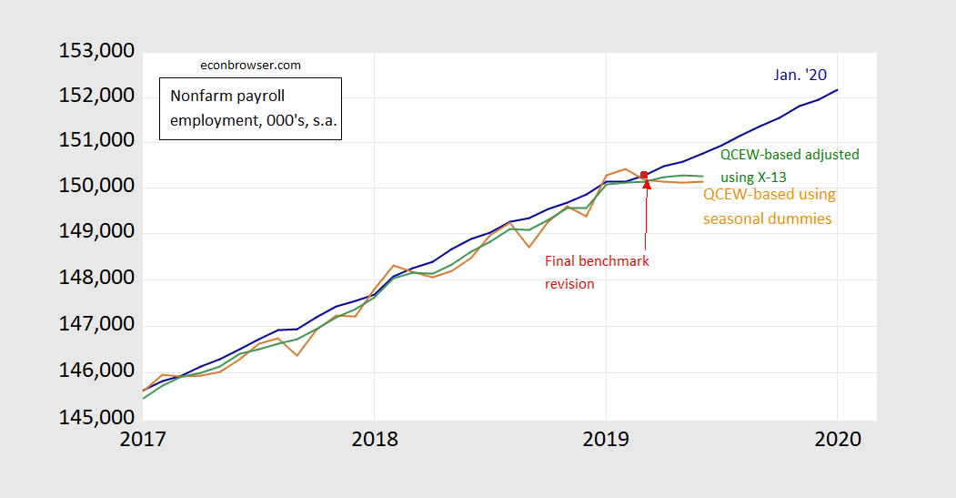
Figure 1: Nonfarm payroll employment, January 2020 release (blue), estimate using log-log regression on X-13 seasonally adjusted QCEW on 2001M01-2019M03 (green), estimate using log-log regression on QCEW with seasonal dummies on 2001M01-2019M03 (brown), and final revision for March 2019 (dark red square). Source: BLS via FRED, BLS, and author’s calculations.
The data used to generate Figure 1 are here.
If you read the documentation for the benchmark revision, you’ll see that the data after March 2019 data is characterized as “post-benchmark”, meaning that really the substantive change is to the level — not contours — of employment.
Without more recent QCEW data, we can’t estimate an alternative trajectory of employment after June 2019.
So, Menzie, you know as per usual I’m a little slow on these things, which number do you take more faith in, the X-13 number or the number using just the regular dummies?? Or is it the old deal where you’d split the difference??
I put a heavy amount of faith in your judgement Menzie, but even you have to concede 505k is a HUGE number is it not?? Or is that a standard number for a revision??
Menzie must slap his head when I ask some of these questions, I honestly didn’t remember him already addressing this until I was looking at the prior post when he was trying to make this easier for some of this doing these regressions/models:
“The preliminary benchmark is not the last word, of course. However, the negative half million revision is larger in absolute value than typical, according to Oxford Economics’ Gregory Daco.”
So, my thought, as far as being on the large end (aside of accuracy in whatever number) for a revision, was semi-confirmed.
*aside from
Moses Herzog: Hard to say one is more reliable than the other – X-13 probably handles seasonality better, but doing a 2-step procedure is probably less efficient than estimating using seasonal dummies.
I am glad that I am not the only one who is questioning the sudden re-acceleration shown in jobs beginning in May 2019 in the latest revisions.
Here’s a graph of the quarterly % change in goods vs. service jobs for this expansion:
https://fred.stlouisfed.org/graph/?g=q7fJ
Goods producing jobs are at a virtual standstill. In fact, ex-construction they are down YoY. Meanwhile job creation in service providing sector suddenly and anomalously (?) accelerated beginning in May of last year. Meanwhile, if you look at the YoY changes in, e.g., the American Staffing Association’s Index of temp jobs, they worsened beginning in autumn – which is not shown at all in the latest BLS revisions.
Like you, I really want to see what the Q3 QCEW is going to show. I suspect it will be a lot softer than the latest BLS revisions.
I am glad that I am not the only one who is questioning the sudden re-acceleration shown in jobs beginning in May 2019 in the latest revisions.
Here’s a graph of the quarterly % change in goods vs. service jobs for this expansion:
https://fred.stlouisfed.org/graph/?g=q7fJ
Goods producing jobs are at a virtual standstill. In fact, ex-construction they are down YoY. Meanwhile job creation in the service providing sector suddenly and anomalously (?) accelerated beginning in May of last year. To the contrary, if you look at the YoY changes in, e.g., the American Staffing Association’s Index of temp jobs, they worsened beginning in autumn – which is not shown at all in the latest BLS revisions.
Like you, I really want to see what the Q3 QCEW is going to show. I suspect it will be a lot softer than the latest BLS revisions.
Professor Chinn,
Using seasonally adjusted data, I find a possible mean adjustment of June 2019 PAYEMS at -484,000 compared to your adjustment of -505,000. I show the 95% confidence range between -102,000 and -865,000.
I show the forecast of June 2019 PAYEMS much closer to the January 2020 PAYEMS data using QCEW data and seasonal dummies as independent variables in a log-log model. I must have an error in my seasonal dummy model that I can’t seem to see. I will move to the back of the class and be quiet.
Hahahaha, you cracking me up dude. I’m still trying to figure out how to define my work directory “wd” so I can import the .xlsx into my Rstudio. I don’t even know if it’s going to work since I usually open it with Mac’s “Numbers” and I don’t have Excel installed. What is Menzie going to do with a guy who hasn’t defined his work directory if he sends you the the back of the class?? I was already here “auditing” the class. hahahaha. I hope Menzie isn’t hiding some heavy brick underneath his podium.
Moses,
You may want to try to get a copy of the EViews student edition, which is quite affordable. It has some limitations on file size and saving files, but you will be up and running in no time. No need to code or program although you can write programs for EViews. Several texts are available showing how to use EViews as related to econometrics and various YouTube videos are available.
@ AS
I’ve made enough effort with the “open ware” or “free ware” I just feel there’s no turning back now. In reality what’s probably holding me back more is my econometrics knowledge. If Menzie hadn’t mentioned “log-log” regression at least once (which he already did in the footnotes) would I have had ANY idea what type regression/model to run?? Possibly…… after maybe 3 days of googling similar model questions, but even that’s a stretch. But not just looking at the variables and problem-solving on my own. I’m telling on myself but that is the reality.
When you try to solve these problems in real life (which is why Menzie’s Uni students may or may not see him as a “gruesome” dude) there is no magical angel is going to whisper over your shoulder “this is a log-log regression set-up to create your OLS”. when the government quotes funny looking employment numbers and you don’t know why.
AS: Did you estimate log-log relation over 2001M01-2019M03 period?
Professor Chinn,
I had used the period 2001m01 to 2019m06 for my forecast.
dlog(payems) @expand(@month) dlog(payems_qceq)
As shown, I used a log-log seasonal index model using the @expand(@month) command and no constant. The @expand(@month,@droplast) command along with a constant shows the same results
Changing to the period 2001m01 to 2019m03 did not make much difference. Using seasonal dummies and the 2019m06 terminal date, I got a June 2019 forecast of 150,622,800. Using the terminal date of 2019m03, I got a forecast of 150,615,200.
oops a “qceq” gremlin got into the titling of “qcew”.
Professor Chinn,
As you suggested, using data from 2001m01 to 2019m03, I find an expected difference in PAYEMS for June 2019 at -511,000 compared to your -505,000. Perhaps the difference is the seasonal adjustment method, I used the automatic X-13 method. I used a log-log model and the residuals are stationary. Am I correct to conclude that the data sets are cointegrated?
1.96 times my SE is 392,000, so my 95% confidence range is similar to yours.
Using seasonal dummies and a log-log model the residuals do not appear to be stationary to me. That is why I used the dlog model.
Pretty good paper and quite comprehensive look for the size of the paper:
https://www.federalreserve.gov/econres/feds/files/2019065pap.pdf
They said on some other sites the “suppression” of some of the data is a problem with QCEW. I feel overwhelmingly relieved to know that in the current 2020 environment where people have privy to what underwear you’re wearing because you signed that away to use a phone app, that corporations are still allowed to keep their privacy. Someone call Justice Roberts and Justice Thomas to tell them thanks.
Household employment definitely leads the unadjusted NFP. It burst until October, so total employment has been flat since October which suggests unrevised NFP will slow down in March-May period.. Adjusted, I think a 200-300 downward revision is likely for 2019
See, I like to think I’m above average intelligence, but sometimes the reality is uh, well I’d rather not say…..but amongst figuring how to import .xlsx into my RStudio (which I haven’t tried yet but think I have a rough idea the steps now and defining my “wd” or “pointing it” there, I was looking at this going “I don’t even know where the start on this as far as making an equation for the R or choosing the package to run”. But Menzie (as usual) throws us a a bone and says it’s a “log-log regression” so, being the rocket scientist you’ve all come to know and love on this blog, it dawns on me I should do a Google search on log-log regressions. So…. it looks like you’re taking “non-linear” data (the employment numbers can vary widely (“volatile” even??) based on the date and which employment gauge, and turn that into a linear number that kinda slices through or “fits” along the general increasing pattern of those “non-linear” data points yeah?? Kinda sorta?? I mean my terminology is probably pretty crappy here, but I think I got a rough idea. Now….I just gotta figure out how the equation looks, but you’re “by definition” going to have log on both sides of the equation yeah??? If I can deduce the exact log-log equation on my own, then get the right “R” package, I think I’m actually closer on this one then I’ve EVER been, especially once I figure out the “import” thing, because it saves me the 6 million years to fill in the spreadsheet cells with the data points. What an “epiphany”.
You’ve now been taken into the internal workings of the mind of a slow person, soon to be used in textbooks on how to deal with developmentally disabled children.
moses, just keep in mind many times when you talk about a log-log regression, what you are really doing is transforming a power law relationship (y=bx^m) into a linear equation. the old adage you learn in school is when you have a bunch of scattered data and you need a simple linear line, do a log transform. however, it is most easily understood as describing the original data with a power law. also helps if the transformed data follows a lognormal distribution. students are constantly amazed by this simple trick rather than learning how to do a nonlinear regression. but then they turn around and do the nonlinear regression on matlab anyways!
I forgot that Buck Henry had passed away. I always thought he was underrated. He did a PBS series on trains when he was half washed-up career wise. Had a comedic style similar to Albert Brooks. Kind of a dry poking fun of life and that there was no owner’s manual for living life:
https://www.youtube.com/watch?v=yOqNLflYYHY
He also claimed some of his screenwriting had been ripped off. A lot of gray area on what actually happened. I suspect that if the film projects hadn’t sold any tickets the parties involved would have insisted it was the other guy who wrote it. There’s no doubt Henry was a great comedic writer either way.
Could this be an odd result of seasonal adjustments that were way off? I’m confused by the economic data these days. It’s getting more confusing all the time.
Job opening data is odd this month as well. Openings plunged without any apparent increase in hiring. Apparently businesses don’t think they need those extra people after all. The job market still looks reasonably healthy, so there’s no panic. But, it sure is a curiosity, and one more thing that’s confusing.