There are various ways of estimating potential output. I typically refer to the CBO’s estimates, which are basically a production function approach (use trend labor and capital stock, and total factor productivity growth, to infer potential output). However, An alternative is to examine price pressures to infer potential output, as in Ball and Mankiw (JEP, 2002).
This is a particularly critical question, given the debate over the desired Fed funds rate, even when just operating within the Taylor rule framework, as discussed in this post.
There are a variety of other methods than the CBO’s (which is essentially a production function approach), including statistical detrending methods such as the Hodrick-Prescott filter (see [1] [2] [3]). Here, I am going to use economics to infer the output gap and hence the level of potential GDP, i.e., exploiting the expectations-augmented Phillips curve, as recounted in this post.
The methodology follows that forwarded by Ball and Mankiw (JEP, 2002), which involves inverting a simple expectations-augment Phillips Curve (without supply shocks, but allowing for random shocks), and assuming adaptive expectations (consistent with the accelerationist hypothesis).
(1) πt = πet – a(Ut-U*t) + vt
(2) Δ πt = a U*t – a Ut + vt
(3) U*t + vt/a = Ut + Δ πt/a
Notice that NAIRU plus a random error is equal to actual unemployment plus the change in inflation divided by a. This suggests that NAIRU can be estimated by filtering the object on the right side of the last equation.
I follow the same procedure, replacing NAIRU with potential GDP, and using core personal consumption expenditure deflator inflation (q/q at annualized rates) for π.
(4) y*t – vt/a = yt – Δ πt/a
I estimate the analogous a parameter over the 1967Q1-2002Q4 period (so I’m assuming the accelerationist model holds over this sample); the estimate I obtain is approximately 0.08. (See this post for an earlier implementation.) I then make two assumptions. First, that adaptive expectations hold, and second that expected inflation equals 2% over the 2003Q1-2015Q3 period — which is pretty close to the average 1-year-ahead CPI inflation rate reported by the Survey of Professional Forecasters over this period, as discussed in this post. In other words, in this second case, I am assuming that inflation expectations are now well-anchored. Hence, the variable on the RHS of (4) is:
(5) yt – (πt-0.02)/a
I then HP filter this variable using the default smoothing parameter for quarterly data suggested by Hodrick and Prescott, to obtain an estimate of potential GDP shown in Figure 1, with green line corresponding to adaptive expectations and red line to anchored.
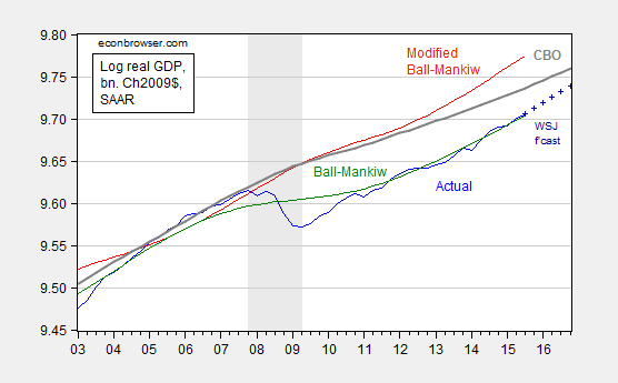
Figure 1: Log GDP (blue), mean forecast from October Wall Street Journal survey (dark blue +), potential GDP as estimated by CBO (gray), and an estimate of potential GDP estimated by use of a modified Ball-Mankiw (2002) method under accelerationist assumption (green), and under anchored inflation expectations (red), all in bn.Ch2009$ SAAR. NBER defined recession dates shaded gray. Source: BEA 2015Q3 advance release, CBO, An Update to the Budget and Economic Outlook (September 2015), NBER, and author’s calculations.
The CBO estimate of potential implies an output gap of -3.2% (in log terms) at 2015Q3. Using the October Wall Street Journal survey estimate for growth over the next year, the gap will still be -2.1% as of 2016Q4! Now, if one believes that the simple accelerationist model of inflation holds (i.e., today’s inflation rate equals last period’s), then the output gap is essentially zero. However, if one believes that inflation expectations are pretty well anchored at 2% (which seems reasonable, given Figure 1 in in this post), the the output gap is nearly -7%! That seems implausible to me, but then, so too does a nearly zero gap, given the lagging inflation rate.
or GDP has been undercounted between 2013-15 and potential overestimated. What happened in the 3rd quarter with the surge in labor costs doesn’t support this level of output gap.
Would it also be possible to set up the Ball-Mankiw model as a UC model and estimate potential with a Kalman filter?
Ernie Tedeschi: I suspect the answer is yes; probably something like Watson‘s (2014) approach.
Today’s JOLTS report suggests we’re pretty close to full employment.
http://www.calculatedriskblog.com/2015/11/bls-jobs-openings-increased-to-55.html
Rosenberg’s analysis of labor force participation rates suggests that workers who have left the economy are not coming back. (See CR, http://www.calculatedriskblog.com/2015/11/rosenberg-on-labor-force-participation.html)
Given that our 15-64 emp to pop rate is well below that of, say, Germany, I am perhaps a bit more cautious, but barring policy changes, Rosenberg may be right.
Is so, then potential GDP growth would be limited to population and productivity gains. I would say, therefore, that some notion of a large output gaps hinges on the assumption of some catch-up in productivity growth, which has been lackluster at best since 2005.
So I put it to you, Menzie:
– Do you think we are at or near full employment?
– And if so, do you believe there is some reservoir of untapped productivity growth?
http://www.cfosurvey.org/2015q3/Q3-2015-US-KeyNumbers.pdf
Take the CFO survey data above, including the anticipated 3.3% wage and salary growth (~43% of GDP) and “health” care spending of 7.5% (20% of GDP, $10,000 per capita, half equivalent of private and public wages and salaries, ~100% equivalent of federal gov’t spending, and TWICE corporate profits after tax), and then take the differential change rates of each to final sales, and the real increase in “health” care spending effectively cancels out (absorbs all of) the real gains in wages and salaries.
That is, the vast majority of firms and workers are laboring each day, day after day, for the “health” care sector, and by extension for the hyper-financialized, gov’t-sponsored- and -protected medical insurers.
Another way to put it is that “health” care spending and insurers’ revenues are capturing all gains of earned income, which was recessionary in 2007-08 and 2000-01 (see below).
http://singularityhub.com/2015/11/10/exponential-medicine-healthcare-is-broken-heres-how-we-are-going-fix-it/
https://research.stlouisfed.org/fred2/graph/fredgraph.png?g=2xVR
https://research.stlouisfed.org/fred2/graph/fredgraph.png?g=2xXy
So, as in the case of total annual net flows to the financial sector absorbing virtually all of US value-added output of firms and labor, “health” care is exacerbating (benefiting from) the hyper-financialization of the economy by taking its marginal share of blood from an increasingly larger bloodless stone/turnip.
“Health” care (and hyper-financialization) is making the US economy gravely ill.
https://research.stlouisfed.org/fred2/graph/fredgraph.png?g=2wlQ
https://research.stlouisfed.org/fred2/graph/fredgraph.png?g=2wlO
https://app.box.com/s/h0p6s4ye96k6cx7smn0r2te0giganyy1
https://app.box.com/s/xcult10g1qfq3qi9wobow4j4l6j0pu0o
https://www.youtube.com/watch?v=vAI2QOBMlTA
https://www.youtube.com/watch?v=CNdOsL4Xe7Q
One cannot earn (?)/receive a Ph.D. from the Ivy schools or Harvard of the West with this kind of thinking/analysis, but thank goodness for that, eh?
One thing I have been curious about is why potential GDP in the quarter and quarters leading up to the beginning of the great recession is equal to actual GDP. Shouldn’t either (a) potential GDP in those quarters be lower than actual GDP given that actual GDP was in a bubble, or (b) the potential GDP line be shifted down after the recession to reflect the fact that potential GDP was reflecting a bubble in the quarters leading up to the recession? For all we know, current actual GDP is equal to what we would be estimating as potential GDP if the economy did not grow at bubble-like speeds in the pre-recession time period.
Just curious, I am sure there is a simple explanation to this.
It doesn’t make sense to argue that there was a supply-side bubble. If resource were in use to produce houses, then those resouces existed prior to the crisis and, unless they have disappeared or deteriorated, they exist now. The housing bubble represented mal-distribution of resources. We were producing the wrong mix of GDP, not more GDP than could be produced by the then-existing resource base, which is what a supply-side bubble would have to be. Put those same resources fully to work in a less distorted distribution, and we could produce the same amount of stuff, but that amount would include fewer houses.
fewer houses, and more bridges, highways, rail and schools would have been a better mix.
“That seems implausible to me, but then, so too does a nearly zero gap, given the lagging inflation rate.” – Menzie Chinn
The gap can be closed with weak inflation pressures.
Just hold down labor power, spread underemployment among more people, reduce labor share by 5%, mute investment and increase inequality. You weaken consumer power for more people.
Now the real problem in understanding low inflation at a zero gap is thinking there is still much more spare capacity with so much underemployment. That is not good thinking. Underemployment does not necessarily imply spare capacity. It could also imply economically marginalized people working in underemployed jobs.
The economy has a balance for the number of labor hours needed for the concentrations of consumer wealth in an economy. The higher concentrations of wealth that we see now imply fewer labor hours in balance. We have seen labor hours peak at the same level for two decades now. The result is that many people will be cut out (marginalized) from the economy because they are not needed in the balance. So what appears as spare capacity is really unneeded capacity that will not be utilized.
hi menzie,
very interesting.
how do you compute a ?
I understand how one can do it with the nairu, regressing delta pi over a constant and the u rate.
i don’t understand it for y since y* is not constant.
furthermore, it does not seem right to use a from the nairu regression for y*since it would imply an identical elasticity of inflation with respect to u gap/gdp gap (which would contradict okun’s law)
rafaminos: I assumed that y* was well measured by the CBO for the 1967-2002 period.
allright, thanks
I think, the labor market has changed too much in recent years for adaptive expectations to hold in the accelerationist model.
It’s uncertain how much of the change in the labor market is permanent or temporary.
Anyway, a small and slow monetary tightening may have a negligible effect on employment.
As in Japan since the late 1990s and early 2000s, today’s U rate is more like the “unnatural” U rate.
Had the labor force grown since 2008 at the trend rate prior to 2007-08, the U rate today would be 13%. Had the labor force grown at the population growth rate, the U rate would be 8-9%.
Thus, by comparison with the post-1970s peak Boomer-induced growth rates of the labor force, employment, productivity (aided greatly by increasing debt to wages and GDP, offshoring, falling energy intensity to GDP, etc.), and incomes, we have a large secular labor “underutilization”, including underemployment of those age 18-34.
Therefore, as in Japan since the late 1990s and the US after the early 1930s (previous secular peaks for debt/GDP), the secular trend rate of real GDP per capita for the “new normal” of “secular stagnation” of the Schumpeterian depression of the debt-deflationary Long Wave Trough will be well below 1%. Take out “health” care spending and net private debt service, and the effect on real spending is a negative average rate of growth since 2007-08.
So, potential real GDP per capita for the post-2007 era is ~0% indefinitely hereafter, which warrants ZIRP. Were outright deflation to become persistent, which is the historical pattern and precedent for Japan and increasingly the EZ, then NIRP becomes the “new normal”.
Despite ample evidence to support the case, the central banksters cannot say this publicly for fear of encouraging a deflationary mindset taking hold among firms and households; but the mass-social adoption of such a position and resulting behavior is rational, as risk of asset, debt, and price deflation is rising along with the implication of low or no returns to financial assets hereafter, which in turn SHOULD encourage risk aversion and liquidity preference for dear liquidity and income.
Thus, the so-called “wealth effect” is largely ineffective (dubious notion in the first instance) during a period of record debt/GDP, low or no returns to financial assets, extreme wealth and income inequality, and a liquidity trap; and the asset bubbles created to encourage the effect become self-defeating because they exacerbate the pernicious effects of inequality, falling velocity and acceleration of velocity, and increasing debt service claims on future growth for many years to come.