On reading my recent post on Kansas economic performance in the reign of Brownback, which included this graph:
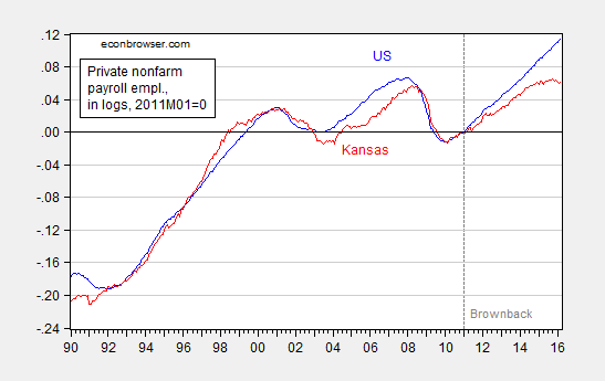
Figure 1: Private nonfarm payroll employment in Kansas (red), in US (blue), in logs normalized to 2011M01=0. Dashed line at 2011M01, Brownback term begins. Source: BLS, author’s calculations.
A&M Professor/Extension Economist Levi Russell writes “Your analysis is highly flawed”.
He then refers me to a post a year ago, critiquing both Paul Krugman’s post “This Age of Derp, Kansas Edition”, as well as my post.
Below the childish title of Paul Krugman’s latest post is a simplistic analysis of the state of the Kansas economy. Krugman references another post by Menzie Chinn that is slightly more sophisticated. I’ll focus on Krugman’s post but will refer to Chinn’s post as well.
…
Since Chinn and Krugman both mention California, let’s have a look at this “boom” in California. For whatever reason (he doesn’t say why he chooses these states), Chinn plots a business indicator from the Philly Fed for California, the US as a whole, Minnesota, Wisconsin, and Kansas. The graph clearly shows faster growth for CA, MN, and the US as a whole than for WI and KS. This is supposed to be a result of fiscal policy and evidence that KS and WI governments (with Scott Walker as its governor) are wrong for implementing right-wing policies.
…
That doesn’t imply, as Krugman states, that we should abandon our skepticism of the effectiveness of gov’t intervention. As I’ve shown here, a more nuanced analysis doesn’t tell the same neat little story about the Wheat State as those told by Krugman and Chinn.
Let me preface my comments by noting it is an honor to be lumped in with Paul Krugman.
One might excuse Professor Russell for not knowing how bad things would get over the year following his post, but in fact he has doubled down on his view that fiscal policy does not explain the evolution of the Kansas economy. In February, he wrote:
… the constant drumbeat from the [Kansas Center for Economic Growth] that the Kansas economy is weak due to the Brownback tax cuts is rather silly. Kansas has had strong private employment growth when compared with neighboring states since the tax cuts have gone into effect. As the recent “Rich States, Poor States” report indicates, two of Kansas’ biggest industries, oil and aircraft, have been under significant stress recently. This is, of course, not caused by the recent tax policy change in Kansas. Agriculture can certainly be added to that list.
Time to look at the data.
First, one cannot appeal to weather, cattle prices, wheat prices, oil prices, or even the aircraft industry’s woes, to explain the Kansas disaster. Consider the following out of sample forecasting exercise. I first estimate an error correction model with Kansas and US GDP over the 2005Q2-2010Q4 period:
(1) ΔyKSt = -8.49 – 0.38yKSt-1 + 0.78 yUSt-1 + 1.46ΔyUSt + 0.002droughtt + ut
Adj-R2 = 0.60, SER = 0.0085, N = 23, DW = 1.77, Breusch-Godfrey Serial Correlation LM Test = 2.07 [p-value = 0.16]. Bold face denotes statistical significance at 10% msl, using HAC robust standard errors. y denotes log real GDP, and drought is the Palmer Drought Severity Index for Kansas (PDSI, lower is more severe).
The data used in this analysis (and for calculations in Figures 3 and 4) are here. Log Kansas and US GDP appear I(1) (fail to reject Elliott-Rothenberg-Stock unit root test) and Kansas PDSI (borderline) rejects a unit root.
Using this ECM to dynamically forecast out of sample in an ex post historical simulation (i.e., using realized values of US and Kansas GDP, and the drought variable), I find that (1) actual Kansas GDP is far below predicted (5.3 billion Ch.2009$ SAAR, or 3.9%, as of 2015Q3), and (2) the difference is statistically significant. This is shown in Figure 2.
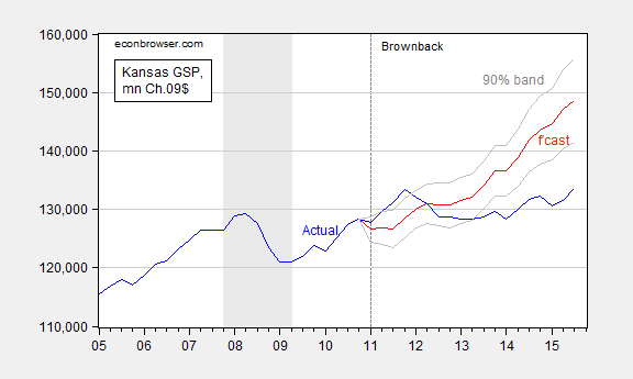
Figure 2: Kansas GDP, in millions Ch.2009$ SAAR (blue), ex post historical simulation (red), 90% band (gray lines). Forecast uses equation (1). NBER defined recession dates shaded gray. Source: BEA, NBER, and author’s calculations.
Note that historical simulation incorporates the effect of drought, despite the fact that the coefficient enters with significance only at the 21% level. In other words, based on historical correlations of Kansas GDP with national, and weather, Kansas should have performed measurably better.
Now, the last refuge the defenders of the Kansas experiment is to say it’s the agricultural or oil sectors, and/or it’s the aircraft industry’s woes, or maybe the plotting of the Illuminati. In Professor Russell’s critique of a Kansas Center for Economic Growth (KCEG) analysis, he uses all three (but omitting the role of the Illuminati).
As the recent “Rich States, Poor States” report indicates, two of Kansas’ biggest industries, oil and aircraft, have been under significant stress recently. This is, of course, not caused by the recent tax policy change in Kansas. Agriculture can certainly be added to that list.
My view: Whenever someone quotes Rich States, Poor States as if it were a source of reliable analysis, watch out!! But let’s take at face value this assertion – it’s anything but fiscal policy.
Let me systematically appraise each of these alternative explanations.
First, re-estimate equation (1) over the entire 2005Q1-2015Q3 period. The drought variable (the Kansas PDSI) does not enter with statistical significance at even the 50% msl. So maybe drought is it, but it doesn’t show up statistically.
Second, substitute in for the PDSI either the real wheat price (CPI deflated), real oil price (core CPI deflated) or the real cattle price (CPI deflated) for the drought variable, and once again the respective coefficients are not significant at the 50% msl, or for cattle is significant at the 50% msl, but with the wrong sign. (Note: log real wheat and cattle prices appear I(1), so I enter in first differences, while PDSI and log real oil prices appear I(0), so I enter in levels).
Hence, one is quickly exhausting the set of possible excuses for the Kansas dropoff.
What about aircraft production? I’ve addressed this in a previous post (Professor Russell shares certain views with Ironman in this regard), but why not repeat? Figure 3 shows a decomposition of growth on a quarter-on-quarter basis (not annualized).
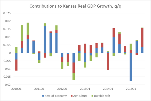
Figure 3: Contributions to real GDP growth, from agriculture (red), durable manufacturing (green), and rest-of-economy (blue). Source: BEA and author’s calculations.
At certain junctures, durable manufacturing and agriculture do subtract from growth; at other times add. But it has been quite some time since these factors have exerted a drag on output growth. Consequently, recent lagging performance cannot be attributed to the factors that Professor Levi highlights.
Finally, what about fiscal policy? Figure 4 shows the correlation between two variables: the gap between actual and predicted Kansas GDP, and the gap between the actual government spending on goods and services and trend (from 2005-2010). Well, as expected, the bigger the shortfall in government spending, the bigger the shortfall in growth.
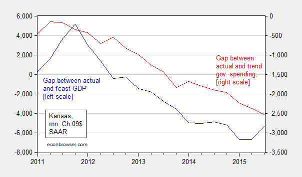
Figure 4: Gap between actual and predicted Kansas GDP (blue), and gap between actual and trend Kansas government spending on goods and services (red), both in millions in Ch.2009$ SAAR. Predicted GDP is from ex post historical simulation using equation (1). Trend government spending is exponential trend over 2005-2010 period. Source: BEA and author’s calculations.
The positive correlation is statistically significant. A regression yields the following result:
(2) Δy_gapt = 5.76 + 2.39Δg_gapt-1 + ut
Adj-R2 = 0.09, SER = 1193.7, N = 18, DW = 0.94. Bold face denotes statistical significance at 10% msl, using HAC robust standard errors. y_gap denotes gap between actual and predicted Kansas GDP, g_gap denotes gap between actual and 2005-2010 exponential trend in Kansas government spending on goods and services.
The slope coefficient is statistically significant at the 6% msl. The confidence interval would encompass the conventional regional multiplier of approximately 1.5 [1]. What’s omitted is tax revenues –- revenues are now down about 2% relative to 2008Q1 peak [0]. That would have exerted an expansionary effect, but since I’ve also omitted transfers, it’s hard to say what the bias would be on the point estimate.
I conclude with my standard graph of GDP growth of the ALEC darlings and betes noire, Kansas and Wisconsin, and Minnesota and California, respectively, because Professor Russell could not discern the basis for my choice of states.
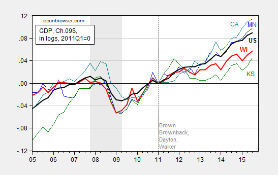
Figure 5: Log Gross State Product for Minnesota (blue), Wisconsin (bold red), Kansas (green), California (teal) and US (black), all normalized to 2011Q1, seasonally adjusted at annual rates, in Chained 2009$. Source: BEA, and author’s calculations.
Notice that pre-recession Kansas was growing faster than the other states and the nation; in the era of Brownback, well, the graph says it all, if you didn’t believe the econometrics.
Digression on fixed effects: At least back in June 2015, Professor Russell made a point of highlighting the difference in extent of slack in the Californian economy vs. the Kansas, arguing that when there is lots of slack, employment growth will tend to be fast. Hence, in his view, the relatively slow Kansas employment growth in Figure 1 is due to the smaller amount of slack, as measured by unemployment. However, apparently, Professor Russell has forgotten about fixed effects. Over the 1976-2007 period, California unemployment is typically about 0.77 percentage points higher than the national average; so the March 2016 California rate of 5.4% is only 0.4 percentage points higher than the national average. By that criterion, California’s labor market is tight. The Kansas situation is the opposite. On average, Kansas unemployment is 1.67 percentage points lower than the national average, and yet, as of March, it is only 1.1 percentage points lower. Hence, there would seem to be more ecnomic slack in Kansas than in California, by this criterion. Given this, the argument that California employment growth is faster because of more slack seems dubious to me. (Additional graphs of CA vs. KS in employment and coincident indices here).
What about Texas?
Also, was not the tax cuts, Government cuts to welfare, social spending, education, and environment, and deregulation suppose to generate an economic “boom” in Kansas and cause business to move their from all over the country and the world? I guess Brownback has not cut enough. I suggest that he shut the universities down except for the basketball and football teams and close the states public schools. We will see how Kansas does after that (perhaps become a center for the private prison industry? Nothing says “libertarian” then “private prison” and the large numbers of chattel workers thereby controlled).
The Kansas tax cut, which took effect in 2013, wasn’t ideal, neither was the tax hike last year, and perhaps some spending cuts. However, every economic recovery is different. Kansas may be near or at full employment. Its unemployment rate matches the 2007 peak – 4.3% – and it’s labor force participation rate is slightly lower than the 2007 peak – 68% vs 70% – which is still much higher than the U.S.. This may be attributed, in part, to its aging workforce. Ironically, Kansas has attracted more low skilled/paying jobs, e.g. in the Leisure & Hospitality Industry, which is booming, although net migration is negative, with slow population growth. Nonetheless, Hispanic net migration is positive.
So Brownback is bringing in W**Backs. That was probably the plan all along.
Someone has to produce for the growing retired population, with lower incomes after retiring, and Hispanics work cheap. That’s been the plan of many politicians.
Menzie,
I agree that one should not use Rich States, Poor States for basically anything. However, when I said that you should be using Colorado as a proxy to show libertarian policies, not Wisconsin or Kansas, you immediately refuted my statement using Rich States, Poor States. Not data. (My suggestion and your response occurred in a previous post’s comment section).
This seems very hypocritical to me!
Colorado implemented TABOR in 1994, which essentially made it more economically conservative than almost any other state in the Union. On top of that, we are quite liberal on drug use and other liberal policies that, when combined with low taxes, would be considered libertarian (not necessarily Republican). I am assuming the reason you do not use Colorado is because it does not align with your bias (though I could be wrong, maybe Colorado is doing terribly when using the methods you show above).
Anonymous: I think there’s a difference between citing RSPS as a valid source of analysis, and citing RSPS rankings as a indicator of what some people think causes growth (e.g., low tax rates, low regulation, etc.) vs. what actually causes growth. In my comment, I was noting the correlation that underpinned the post: namely when ALEC outlook rankings go down, growth is faster rather than slower. In other words, I was re-iterating the failure of RSPS rankings.
I hope that sufficiently clears up matters.
How much of the variance is attributable to tax/spending cuts?
Perhaps looking at the various indicators of unemployment would be better than focusing on U3 alone. http://www.bls.gov/lau/stalt.htm
Kansas and Wisconsin look much more like Minnesota than California which is laboring under a much larger U6.
As an aside, I’ve wondered what GSP as a percent of long term liabilities might look like for the various states. Haven’t been able to find that or even if that make sense, but if growth is fueled by increasing liabilities, is that a good strategy? In Michigan, the state has taken steps to curtail the growth in long term liabilities which seems to have made the state more fiscally sound without huge tax increases. Most of that liability came in the form of generous pensions that were largely unfunded. The idea was in order to get and keep the best, the government had to be generous which mean pensions that were seldom, if ever, matched in the private sector. Of course, there was no evidence that the government ever got the best or that it resulted in greater state economic growth.
Michigan’s House GOP cited these changes http://gophouse.org/wp-content/uploads/2015/02/ActionPlan_2015.pdf:
After four years, we have accomplished nearly every objective we’ve
set out to complete. Some of the highlights include:
Paying down the state’s long-term debt by more than $21
billion to free our children from future liabilities.
Delivering transparent and accountable government, which
produces real, responsible results. For example, turning the
state’s $1.5 billion deficit into a budget that now has more
than $500 million in the state’s Rainy Day Fund.
Phasing out the Michigan Business Tax and Personal Property
Tax to be fair to all taxpayers and job providers.
… among others.
Not sure how Michigan would look in those log charts.
“The idea was in order to get and keep the best, the government had to be generous which mean pensions that were seldom, if ever, matched in the private sector. Of course, there was no evidence that the government ever got the best or that it resulted in greater state economic growth.”
do you have evidence of this claim? often times, government wages were lower than private sector equivalents (not always easy to find equivalents) and the pension covered the gaps. you may be drawing preconceived conclusions from an ideology rather than data.
baffling, it’s possible that “the pension covered the gaps”. As you indicated, “not easy to find equivalents” at the state level. However, the CBO did an analysis at the federal level: http://www.cbo.gov/sites/default/files/cbofiles/attachments/01-30-FedPay.pdf
Except for the highest levels of education, the government compensation was equal to or better than the private sector.
With regard to pensions, I found this for Michigan: http://www.michigancapitolconfidential.com/19248
This has the average pensions for all states: http://www.aei.org/wp-content/uploads/2014/03/-aei-economic-perspective-march-2014_160053300510.pdf
So, I can only conclude that the generally more generous public sector pensions along with roughly comparable salaries indicate the government seeking to be competitive at attracting the best without any evidence of greater economic growth. Or, perhaps, it is just bad stewardship of taxpayer money.
be careful when extrapolating federal to state and local government, especially at the low end. the fed hires alot of less educated people who have to work in secure environments, which significantly changes the pay scale. you cannot pay a janitor working in a classified facility like you would a janitor at mcdonalds.
when you look at the secretary working in the local county engineers office, i do not believe they are making a better living than those in the private sector. you quote an aei study, in itself a rather dubious position defense. aei already has a preconceived agenda. as an aside, and the aei study tries to preempt this argument without success, the problem may not be overly generous public sector pensions, but poorly planned private sector retirement strategies. you cannot compare the private and public sector, and say the public sector is too generous, without doing a thorough analysis of the adequacy of the private sector retirement strategy. it has become very obvious, the switch to 401k type retirement system is severely lacking in long term adequate retirement income for the vast majority of people. you can blame the private sector for not saving enough, but it does not change the fact many retirees in this system are retiring without adequate retirement support. and you should not punish the public sector for this private sector failure.
baffling… or you can blame government for being far too generous with taxpayer money when it comes to pensions. I guess it depends upon which preconceived agenda you have.
The private sector is phasing out fixed retirement plans because they are far too expensive given the array of other benefits and co-taxes businesses have to pay. But affordability has never stopped government from granting more… and more… until now.
Bruce Hall Keep in mind that many state and local government employees are prohibited from receiving Social Security benefits, so a lot of what you see as a pension is in fact just a state and local government replacement for Social Security. This is also true for federal workers hired before 1984. And for those federal workers hired before 1984, if they later choose to go work in the private sector, they must both pay into Social Security and forfeit those benefits. Federal workers hired after 1983 do have a defined pension, but it is MUCH less generous than the old CSRS pensions. And of course federal workers have to contribute to that plan, so it’s not entirely a free benefit. The CBO study mentioned that the federal government pays more in health insurance premiums for its workers. This is true. But the implication is that federal workers must therefore enjoy cheaper healthcare costs. Not quite. In fact, the federal government deliberately overpays for health insurance because it is a roundabout subsidy to keep private health insurers afloat. So everything isn’t always quite what it seems. What the CBO scored as a benefit for federal workers is actually a backdoor subsidy for private sector workers.
Still, I would agree that overall federal government workers enjoy better benefits than private sector workers. This is especially true at the lower grades. Except for overtime. In the private sector workers get time and a half for overtime. In the federal government overtime pay is actually less than straight time pay. Federal government workers are also exposed to significant risks…particularly identity theft risk from unfriendly governments. Also, a private sector worker can quit anytime. There might be civil penalties, but your former employer cannot put you in jail for quitting. Not so with the federal government. It is rarely enforced, but it does happen. Not only that, but if you were once a federal worker who quit and found another job in the private sector, the federal government can come back later and require you to quit that private sector job and return to your former duties. Again, it doesn’t happen often, but it does happen. Ask the workers at Pueblo Army Depot. Here’s another risk. You are free to read WikiLeaks if you want. It’s not a crime. But it is a crime for a federal worker to read WikiLeaks even on his or her own personal computer at home. There are all kinds of crimes that only apply to federal workers. We are constantly having to take refresher training on things that are legal outside of federal employment but illegal if you’re a federal worker. It’s true that federal workers are rarely fired; but that’s because the usual way of getting rid of federal workers is by threatening them with criminal prosecution for violating some obscure provision in law that only applies to federal workers. That’s just how it works. So federal workers have to give up quite a bit in exchange for those greater benefits.
bruce,
“or you can blame government for being far too generous with taxpayer money when it comes to pensions. ”
that general statement has been shown to be incorrect. are there some pensioners with higher payout than deserving? probably so. i know, particularly from my time in florida, there were many police and firefighters who took advantage of loopholes created by babyboomers which characterized pensions based on the last few years of pay which were artificially inflated by overtime. i agree those cases should be subject to fair revision. however, you cannot throw out all these pensions because you do not like the outcome of a few cases. the vast majority of pensions are not overvalued. if you think there was fraud involved, then go back and prosecute the officials who struck the deal in the first place. but wanting to penalize after the fact the worker, who accepted an employment agreement, is not really fair. unless you accept that your own past employers can also claw back any retirement funds they gave you years ago, after determining your long term contributions to the company were not truly worthy of the payout at the time.
Edited:
I don’t really have a position on the macro question at the center of this discussion, but I will say I am confused by the econometric methods you chose to defend your position.
Do you really want to base your argument for whether drought or oil prices “explain” Kansas GDP to be based on whether including these variables in a simple regression improves out-of-sample forecasts? If so, I’m not sure that tells us very much for two reasons. First, there is a difference between “X is a good predictor of Y” and “X causes Y.” Second, the sort of structural approach to forecasting you’re trying has a long history of not yielding very good results. So I’m not surprised your model doesn’t yield good forecasts either. Univariate methods like ARMA models typically do a much better job of forecasting.
Putting that aside, through out the post you seem very tempted to switch from evaluating your models based on their forecasting ability to telling stories about the individual coefficients you estimated. I am not sure that is a good idea for three reasons.
#1.Isn’t ΔyUSt also a function of ΔyKSt by definition? If so, then doesn’t including it as an independent variable introduce an endogeneity problem that biases your coefficient estimates?
#2. Are you sure cattle prices and wheat prices are exogenous to ΔyKSt? If not, you have the same problem as above. I think your assumption that these prices are exogenous is probably true, but it probably depends on how and where these prices are measured. For example, I would be less concerned about endogeneity if they are supposed to reflect world prices.
#3. It seems possible that many of the variables you are including are highly correlated with each other. For example, ΔyUSt might be correlated with weather, oil price, cattle price, etc. yUSt-1 could also be correlated with oil, wheat, and cattle price (since these products are produced over a relatively long time horizon). If that is the case, maybe a t-test on the individual coefficient isn’t the best way to determine if these variables matter or not. The multicollinearity could be pushing up your standard errors making relevant variables appear irrelevant. Maybe a joint-hypothesis test would be better? On a related note, I am not sure why you are just looking at these variables one at a time anyways.
Anyways, these are just my humble thoughts. It looks like this conversation on Kansas covers several lengthy posts and comment threats. I did not attempt to comb through all that discussion, so if you have addressed any of these concerns in a previous post, then I apologize. These are just my concerns about the econometric methods you are presenting in this single post.
DW: These are relevant and excellent questions. Let me answer each in turn.
I agree that it is hard to forecast; however, what I am conducting is an ex post historical simulation (in the language used in the old Pindyck and Rubinfeld textbook). I estimate the model over a sample, reserving some of the sample of out-of-sample validation. I then use actually realized values of the right hand side variables to dynamically “forecast” (really, predict) the dependent variable (first differenced log Kansas GDP) and then integrate up to the (log) levels. With realized (ex post) values of the right hand side variable, the model should do better than a simple ARMA (and in my experience does, except in cases like exchange rates and other asset prices where it is extremely difficult to beat a random walk).
On #1, mechanically ΔyUS and ΔyKS should be correlated, but given the relatively small size of Kansas versus the US, this should be minor. I can bet you that had I subtracted Kansas GDP from US, and used that instead of US GDP, I’d get virtually the same result.
On #2, cattle prices might be endogenous; I suspect that global wheat prices are pretty exogenous. But you are right, I have not conducted a formal test.
On #3, I conducted a formal Wald test for the joint restriction that the coefficients on drought, cattle prices, wheat prices and oil prices are all zero. The F-test fails to reject the null at p-value 0.638; Chi-squared at 0.629.
Thank you, once again, for asking relevant questions. Hopefully, these comments address some of your concerns. In any case, the dataset I use in the analysis is here.
I think these are all fair responses to my questions. The discussion on the difference between forecasting and ex post historical simulation was particularly useful. Thanks for clearing this up.
Slower or less U.S. economic growth likely negatively affect some states more than others. For example:
“When the drought and Great Depression hit in the early 1930s, the wheat market collapsed. Once the oceans of wheat, which replaced the sea of prairie grass that anchored the topsoil into place, dried up, the land was defenseless against the winds that buffeted the Plains.”
Well it’s good to see you graduated from petty name calling to assertions of conspiracy theory. Not much of an improvement, though.
You said to one commenter:
“I think there’s a difference between citing RSPS as a valid source of analysis, and citing RSPS rankings as a indicator of what some people think causes growth”
All I did in my post was cite RSPS, hell I didn’t even cite their rankings! In nearly every post on my blog on Kansas I am careful to point out that I’m not defending Brownback or his policies, merely pushing back against simplistic analysis by a certain think tank in Kansas and by political commentators such as Krugman. You got caught in the mix one time and have gone on a tirade of red herring over it.
What’s interesting to me about this post is that the only data I discuss on my blog are private employment statistics. Everything in this post is about gross state product, yet you plaster my name everywhere. It’s nonsensical.
Your final jab in this post regresses the state output gap on the fiscal gap. You then conclude that there is a positive relation between the two and that this somehow implies that a reduction in gov’t spending is a drag on the economy. I’ll just point out that 1) this has nothing to do with PRIVATE employment and 2) that gov’t spending is a component of GSP. Of course they’re positively related.
What do you have to say about North Carolina? Why hasn’t their reduction in spending caused an economic slowdown?
You seem quite convinced that I’m some kind of ideologue but my short blog posts on this subject have been full of comments about my reservations about Brownback. Perhaps you should stop projecting.
Levi Russell: What name did I call you? Please be specific in your answer. On the other hand, I do seem to recall a comment about me “spouting nonsense”. If that was not posted by you, I apologize for misattribution.
Actually, the post you referred me to cites employment, unemployment rates, and coincident indices; the coincident indices are aimed at tracking state level GDP, if you read the documentation. Hence, GDP seems relevant to me. And in fact, in my post, I start off with a graph of private NFP (that would be Figure 1!), discuss unemployment rates, and coincident indices. So we are talking about the same variables!
Regarding built-in-correlations, it seems useful to move beyond accounting definitions. If the world is Classical, then there is no correlation between government spending and GDP. Depending on the model, one can get positive, negative, or zero, correlation. Please consult a intermediate macro textbook.
Finally, I don’t believe you’re an ideologue. I just believe you are heck-bent on adducing the lagging performance of Kansas to anything, anything, but fiscal policy, when a reasonable person would evaluate the possibility of fiscal effects.
Your response to my original comment on the last post was laden with insults and you know it.
Yes, the first post. You’ve brought the rest of mine into it and referenced them here. None of them dealt with GDP. Since you insist on me reading everything you’ve ever written on the subject, maybe you should read my posts. In them, I insist that KCEG use private employment in their analyses.
My point on GSP was apparently too subtle. Kansas has had fairly dramatic reductions in gov’t spending and GSP has fallen. Again, of course they’re positively correlated. Where’s the demonstration of causation? You have another clear-cut case where the opposite is happening during the same time period in NC. Are there factors at play that you aren’t (can’t?) accounting for? What is the “story” you’re trying to tell here? Why are Kansas’ tax and spending cuts bad for growth and NC’s not?
“I just believe you are heck-bent on adducing the lagging performance of Kansas to anything, anything, but fiscal policy, when a reasonable person would evaluate the possibility of fiscal effects.”
Why do you believe that? Do you know me personally? Why can’t it be that I’m just pointing out other factors at play? Clearly the case of North Carolina throws water on the idea that reductions in gov’t spending are, generally speaking, a drag on economic growth. You seem to want to focus exclusively on the case of Kansas and completely ignore NC. Why?
Levi Russell: Thank you for confirming: (1) I did not call you any names. (2) You characterized my post as “nonsense”.
I think if you are willing to sling it, you should be ready to accept what comes your way.
In regard to your query about NC, I would think that someone who is trying to understand the diverging paths would undertake an empirical analysis. While I haven’t looked at NC before, ten minutes allows one to download NC GDP, government, and create a counterfactual, using a similar methodology as used in this post. The covariation of NC GDP and US GDP differs, and in fact, using historical correlations, predicted (out of sample) and actual differ by less than 1%. So in some ways, there is no “divergence” to explain. On cursory analysis, it does appear that in the full sample, government sector activity covaries (in first difference) with GDP, but not at conventional levels of significance, so no strong conclusions can be drawn.
If you have substantive comments regarding the statistical/empirical evidence contradicting my inferences, on either Kansas or North Carolina, I would welcome seeing them.
So according to you, tax cuts in Kansas have obliterated the economy but not so in North Carolina. What conclusions do you draw from that? Does it make you skeptical about your (perhaps simplistic) empirical analysis? Precisely what is the mechanism that you’re measuring here? I hope you’d agree that ad hoc empirical investigations without theoretical foundations can lead to poor conclusions. At the very least such investigations are not generalizeable.
I had hoped you understood the difference between insulting a person (which you seem to love doing) and commenting on their work in a negative way (which I did). Apparently not.
Levi Russell: In my model, it’s tax cuts combined with a balanced budget requirement (either de facto or de jure) which implies a contractionary effect from tax cuts. If the tax cuts do not reduce the tax burden in a way that stimulates consumption much, or spurs investment much, then the tax cuts are even more contractionary. This is an application of the balanced budget multiplier. I lay out this model in the Wisconsin context here.
As for the definition of insults, if you say I spout “nonsense” (a statement on my analysis), then I think I am justified in making my assessment that your MPL would be higher doing a different activity than economic analysis (also a comment on your analysis, not you as a person).
I have to investigate the NC case, but I thank you for leading me to another case to investigate.
Regarding cross-section investigations — atually, we do have evidence on the size of fiscal multipliers at the state level. I cite a few in my New Palgrave Dictionary of Economics survey on the subject of multipliers.
“As for the definition of insults, if you say I spout “nonsense” (a statement on my analysis), then I think I am justified in making my assessment that your MPL would be higher doing a different activity than economic analysis (also a comment on your analysis, not you as a person).”
It’s just incredible to me that someone with a PhD can’t comprehend basic logic. The proper response to my claim that your analysis is wrong isn’t to insult me (as you’ve done several times) or to say that I’m a poor economist, but to explain why your analysis is right and my critique wrong. You’ve made an effort on that front, but the manner in which you’ve done so is hilariously childish. I may not be an expert on this particular subject, but to conclude that I am a poor economist in general doesn’t follow. The internet is a tough place for people with thin skin.
As I’ve said on my blog, I’m critical of Brownback’s tax cuts. The way he and the legislature implemented them frankly seems silly and reckless. If THAT is your critique, then we agree. It’s certainly possible that the way the tax cuts were implemented could cause short-run economic problems, especially in a state that faces pretty serious demographic issues. It doesn’t follow, though, that increasing taxes solves said demographic crisis. Attempts by some people to compare Kansas with another state simply don’t pass muster as natural experiments. The case of NC is anecdotal evidence that reducing taxes and spending can be good for an economy.
Levi Russell: I don’t see anywhere where you have “clarified” the difference. Please provide a link where I personally insult you, with the quote.
If you want to move to substance, I re-iterate, a positive coefficient between government spending and GDP is not a foregone conclusion. Remember, you stated: “I’ll just point out that …. that gov’t spending is a component of GSP. Of course they’re positively related.” Yet, I have not seen a rejoinder, nor have I seen an econometric critique of my post on Kansas. I was careful to include links to the data source at BEA. The other data are from NOAA or FRED — you can do your own empirical analysis, instead of calling what I wrote “nonsense”.
Now you’ve taken us completely off topic. My original critique well over a year ago had little to do with our conversation in this comment thread.
I’ve provided plenty of critique that is relevant to the problem. You aren’t the sole arbiter of what is relevant, sorry.
Levi Russell: Well, then, please provide an econometric critique of this post that holds water.
“Clearly the case of North Carolina throws water on the idea that reductions in gov’t spending are, generally speaking, a drag on economic growth. ”
that was the case nationally with austerity measures. we saw the same drag in europe with austerity measures as well. seems that would require throwing a lot of water to refute.
Start with real GDP by state from the BEA link, and fill in any missing 2014 industry level detail with a first cut assumption of 2014=2013. Kansas all industry total (line 1) increased 3.7% from 2010 to 2014. US all industry total increased 7.0%.
Now from the all industry total (line 1), subtract other transportation equipment manufacturing (line 22), Federal civilian (line 83), and Federal military (line 84). Essentially, this measures overall less aircraft manufacturing and Federal. From 2010 to 2014, this truncated measure of state output rose 6.4%. For the nation as a whole, this same truncated measure rose 7.6%.
Abstracting from aircraft and Federal then – things a state’s governor has little control over – the shortfall of Kansas growth relative to US during these four years was 1.2%. But the slump in aircraft and Federal will, through the multiplier effect, also shave growth off other sectors. Hence when taking this secondary effect into account, the relative shortfall will be even less. Thirty other states, in fact, have lower truncated growth (per the above construction) than Kansas. While not one other state has a within-state total-vs.-truncated discrepancy of this magnitude. Kansas has a unique two-prong problem.
“Notice that pre-recession Kansas was growing faster than the other states and the nation; in the era of Brownback, well, the graph says it all, if you didn’t believe the econometrics.” Let’s call pre-recession from 1997 to 2007. The Brownback era is the four years 2010 to 2014. For the nation as a whole, the Federal sector increased a cumulative 3.2% over the ten pre-recession years. In Kansas it rose a far greater 16.0%. For the nation, Federal fell a total of 4.4% during the Brownback years. In Kansas Federal fell a far larger 11.7%. Of course the graph does not say it all. If anything it obfuscates, since it takes no cognizance of the significant changes that have taken place beneath the surface in Kansas that are beyond the state’s control.
There’s more. The 2008 crisis induced abnormal structural change. This, however, did not stop the economy from rebounding from its cycle trough. Here are US real GDP growth rates (4thQ to 4thQ) for 2009 (-0.2%), 2010 (2.7%), 2011 (1.7%), and 2012 (1.3%). The rebound in 2010 is a natural consequence of the transitory inventory rebuild. All states have such a rebound. But as inventories equilibrate, states with weightier structural change that’s starting to play out will soon see their growth rates (and employment gains) taper off relative to the national average. This is what happened in Kansas, and it has little to do with who held the governorship. What’s especially fraught with risk is trying to explain what is going on with an equation like (1) that includes simple one-quarter growth lags. Such an equation produces coefficients derived from comingled data coming from two distinctly different structural time periods, additionally whipsawed by a powerful cycle. It’s like making a milk shake with chocolate ice cream and asparagus. Yep, you’ll get statistical results. After all, the raw data are just numbers that are clueless about their dates. But who would want to drink such a concoction?
Kirk asks, what about Texas? Cumulative growth during the 2010-2014 period was 21.0%. Falling to 17.7% after excluding natural resources and mining. Texas has a far more diversified economy, however, making this kind of analysis much more complicated than that of Kansas. Right off, Texas per capita growth was 13.4%. So it’s evident Texas state product benefited hugely from population growth. Some of this was due to oil, some of course due to heavy contiguous-to-Mexico immigration that has built over time.
How does an economist separate wasteful and inefficient spending from GDP? If a state wastes money it will create jobs and increase GDP. If a state cuts waste if lowers GDP and jobs. Wasting money should have a long term consequence while efficiency should not.
Waste is never good. How can it possibly be? The more that money disconnects from the real sector, the more the waste. The more government involvement, the more the waste. Economists do not separate wasteful projects from productive ones. This is the task of the market. Bringing me full circle. The more money-disconnect and the more government-intrusion, the less efficient markets will be, the more waste there will be, and the slower the growth of the standard of living average Americans will be. If politicians feel they have good reason to interfere, each and every project without exception should be subject to full disclosure and cost benefit analysis by an independent private panel. Rare is the government official who can be trusted in this day and age to hold down waste Rarely even still are government cost-benefit analyses. It is corruption to the left, corruption to the right, and corruption straight down the firing line …
implied in your argument is private sector spending is always more efficient than public sector spending. not sure if this view is justified to the degree asserted. for instance, teachers are extremely productive when compared to their salary costs. in the majority of schools across the country, teacher pay is probably of a cost return that few in the private sector can truly match. we simply have very poor economic models to value the work of a teacher. in this case, cutting a teaching position to return that money to the private sector will probably produce less efficient returns.