The cumulative growth gap since January 2011 between the US and Wisconsin coincident indices was 2.2% in December. The forecast indicates a continued widening to 2.8% in six months time.
Figure 1 depicts the log coincident indices for Wisconsin and the US.
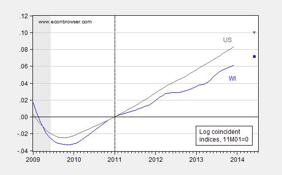
Figure 1: Log coincident indices for Wisconsin (blue) and US (gray), and levels implied by leading indices for 2014M06. NBER defined recession dates shaded gray. Source: Philadelphia Fed, NBER, and author’s calculations.
Reader Ed Hanson wonders about the predictive characteristics of the leading indices produced by the Philadelphia Fed. Figure 2 depicts the actual and forecasted six-month growth rates for Wisconsin.
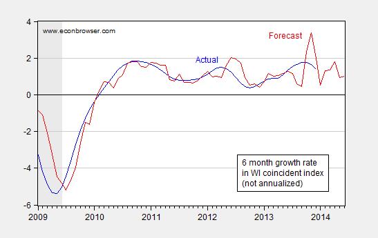
Figure 2: Actual six-month growth rate (non-annualized) in WI coincident index (blue) and corresponding leading index (red). NBER defined recession dates shaded gray. Source: Philadelphia Fed, NBER, and author’s calculations.
A regression of the actual six-month growth rate on the forecasted yields the following results:
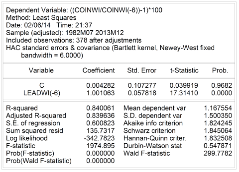
Table 1: Unbiasedness test.
Note that the leading index appears to be an unbiased predictor of actual six-month growth rates, since the point estimate of the slope coefficient is 1.001, with a Newey-West robust standard error of 0.058; hence one would not reject a null hypothesis of a unit coefficient. The adjusted R2 is 0.84 — in other words 84% of the variation of the six-month growth rate around the mean is explained by the leading index. Note that this is not a “real time” analysis, as the coincident series are the revised, rather than initial, figures, and one might wish to compare the forecasts to the initial.
The leading index for the United States shares the same characteristics of unbiasedness; the adjusted-R2 is 0.93.
Has the behavior of the Wisconsin index changed over time? The log ratio (WI/US) rose from 1982 to a peak in 2000 before descending. Estimating the relationship between the (log) WI coincident index and the (log) US coincident index using dynamic OLS (6 leads and lags of the first differenced right hand side variable, 2001M01-13M12) and a dummy taking a value of one from 2011M01-2013M12 yields a cointegrating coefficient of 0.507, and the coefficient on the dummy is 0.021, significant at the .0002 level using Newey-West standard errors. Literally interpreted, Wisconsin economic activity is 2% lower than usual, starting from 2011M01.
This is not a conclusive finding; using a different specification, sample period, or estimation method would likely lead to a different finding.
Update, 2/8 noon Pacific: Reader Ed Hanson still contends that Wisconsin economic performance has improved since 2011M01. He writes:
What we mainly disagree with, the Walker policies have began the change back toward superior economic performance. I say it has, and comparing the performance of Wisconsin from 2001 until 2011, with Wisconsin after 2011, supports my position. In addition, Walker policy of reduced taxation, both personal and business, since 2013 will accelerate economic performance.
Since Mr. Hanson is not persuaded by a coefficient on a dummy variable, I have undertaken another analysis, which conditions on US economic activity, and lagged WI economic activity. I estimate a error correction model over the 2001M01-2010M12 period:

Table 2:Error correction model, WI and US economic activity.
Where LCOINWI (LCOINUS) is the log coincident index for Wisconsin (United States), “D” indicates first difference. Note the high adjusted-R2, Q(6) and Q(12) statistics fail to reject the no-serial correlation null, as does the Breusch-Godfrey LM (2 lags) test.
The implied long run cointegrating coefficient is approximately 0.50; that is a 1 percent increase in the US coincident index is associated with a 0.5 percent increase in the Wisconsin index, over the 2001M01-2010M12 period.
I use this error correction model to forecast out of sample (2011M01-2013M12), conditioning on actual US economic activity. The forecast is shown in Figure 3, with plus/minus two standard errors, compared against the actual.
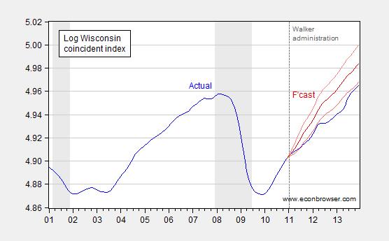
Figure 3: Log actual WI coincident index (blue), forecast (red) and plus/minus two standard errors (pink). Forecast based on error correction model (Table 2). Dashed vertical line at beginning of Walker administration. NBER defined recession dates shaded gray. Source: Philadelphia Fed, NBER and author’s calculations.
Notice that the actual Wisconsin index under-performs the forecasted (what we would call the counterfactual, if the usual economic relationship between the US and WI economies prevailed into 2013) by a significant amount — by up to 2.5% (log terms) earlier in 2013, and 1.9% as of 2013M12. The fact that the blue line (actual) is outside of the plus/minus two standard error bands suggests that the under-performance did not happen by accident, at conventional significance levels.
Walker is pretty quiet about his economic and jobs performance. Too busy running around the country collecting huge donations to do anything for the people of Wisconsin.
Another schadenfreude post by Wisconsin’s self-appointed critic. It is sad when those who do not live in Wisconsin have to defend it agains those who do even when they find their taxes reduced because of effective government.. Why do such people still live in a state they hate?
BMO forecasts growth for Wisconsin economy
Excerpt:
Wisconsin budget surplus hits $977 million
ricardo, my aren’t we defensive!
menzie is simply showing that wisconsin is lagging behind the overall us performance. hence its local performance below par may be attributable to local policy (aka walker) rather than federal policy (aka obama). since overall us performance is increasing, one would also expect that to happen in wisconsin as well. just saying it does not seem to be doing as well as the country as a whole.
Not sure that Wisconsin is all that unique with regard to it’s economy. It’s all what you measure. You can measure manufacturing, goods & services, and employment and probably get different pictures. What appears to be the case is that there is no significant labor improvement anywhere in the Midwest.
Wisconsin
2013
Labor Force Data
Civilian Labor Force (1)
3,077.3 3,071.2 3,071.7 3,065.1 3,068.6 (P) 3,071.7 … DECLINING
Employment (1)
2,867.5 2,865.6 2,869.3 2,866.6 2,873.7 (P) 2,880.3 …GROWING
Unemployment (1)
209.8 205.6 202.4 198.5 194.8 (P) 191.4 … DECLINING
Unemployment Rate (2)
6.8 6.7 6.6 6.5 6.3 (P) 6.2 … DECLINING
Illinois
2013
Labor Force Data
Civilian Labor Force (1)
6,540.6 6,525.5 6,527.1 6,519.5 6,522.7 (P) 6,538.7 … FLAT
Employment (1)
5,936.0 5,923.6 5,935.0 5,940.2 5,955.4 (P) 5,973.5 … GROWING
Unemployment (1)
604.5 601.8 592.0 579.3 567.3 (P) 565.3 … DECLINING
Unemployment Rate (2)
9.2 9.2 9.1 8.9 8.7 (P) 8.6 … DECLINING
Michigan
2013
Labor Force Data
Civilian Labor Force (1)
4,727.7 4,727.1 4,736.3 4,723.9 4,706.5 (P) 4,694.3 … DECLINING
Employment (1)
4,309.4 4,302.5 4,311.7 4,300.7 4,293.4 (P) 4,300.1 … DECLINING
Unemployment (1)
418.4 424.7 424.6 423.2 413.1 (P) 394.2 … DECLINING
Unemployment Rate (2)
8.8 9.0 9.0 9.0 8.8 (P) 8.4 … DECLINING
Minnesota
2013
Labor Force Data
Civilian Labor Force (1)
2,978.5 2,970.5 2,968.9 2,964.6 2,966.0 (P) 2,971.6 … DECLINING
Employment (1)
2,824.6 2,818.0 2,821.0 2,822.2 2,828.3 (P) 2,834.2 … GROWING
Unemployment (1)
153.9 152.5 147.8 142.4 137.6 (P) 137.3 … DECLINING
Unemployment Rate (2)
5.2 5.1 5.0 4.8 4.6 (P) 4.6 … DECLINING
Professor Chinn,
Could you comment upon whether the example you present is an example of cointegration, since one would not think coincident indicators would wander too far from actual? Also, could you comment upon the Durbin-Watson statistic? My understanding is that for univariate analyses, one likes to see a Durban-Watson statistic have a value of about 2.0 to indicate that residuals are not correlated. What is the interpretation of the Durbin-Watson statistic for your two variable example? Some additional comments about the Newey-West standard errors and the Wald F-statistic would also be appreciated. Thank you.
Bruce Hall: Since you commented on this post, I would have thought you would have refrained from looking at comparisons of month-to-month changes — I am comparing multi-year trends. The data are available at the Philadelphia Fed, so I leave it up to you to calculate the trends for the regional economies, as I did before.
AS: The regression output reproduced in the post does not pertain to a cointegrating regression; rather it is a regression of an actual growth rate on a forecasted growth rate. The low Durbin-Watson statistic is indicative of serial correlation in the regression residuals. Since the forecasts are overlapping (six month changes while the data frequency is monthly), then under the null that the forecasts are efficient, the regression residuals should be serially correlated, specifically MA(k-1).
In contrast, the dynamic OLS (DOLS) regression I discussed does pertain to a cointegrating relationship. Depending on the trend specification, a Johansen multivariate approach indicates cointegration at the 10% significance level. The DOLS regression does produce a R2 greater than the DW statistic, but since I pre-tested for cointegration, I don’t put heavy reliance on the Granger rule-of-thumb.
Professor Chinn,
Thanks, I seem to need more reading on the proper definition of cointegration and distinction between actual growth on forecast growth and cointegration. Would the forecast you made be enhanced by adding an MA(k-1)j term?
AS: The leading indices and the growth rates are integrated order zero by typical ADF tests — so no need to do a cointegrating regression. The WI and US coincident indices are I(1) processes; hence, one would want to apply some cointegration methodology to those series, which is why I use the DOLS regression procedure in that case. See this old paper for a cookbook approach.
The induced MA process (under the null) does not bias the point estimate. However application of the standard formula for the standard error would lead to biased estimates, so that’s why I use the robust standard errors in that regression. See Hansen and Hodrick (1980) on the subject.
I’ll be presenting on supply-constrained forecasting at Columbia University on Tuesday.
The blurb and registration: http://energypolicy.columbia.edu/events-calendar/global-oil-market-forecasting-main-approaches-key-drivers
260 have signed up so far.
New York investors in oil and gas will be interested in this one.
Professor Chinn,
Thank you.
Menzie
The question from me you answered was not exactly what I asked or, perhaps, what I meant to ask. I was leading more toward a correlation of the coincidence index at time of major policy and tax changes to predicting the change either of gross state product or employment numbers. But regardless as usual I found your work quite interesting, and I thank-you for it.
Figure 2. From your notes and looking at FRED, I understand you moved the leading indicator graph forward six months to correlate the predicted CO Index. Noting that you properly informed us readers that coincident series are the revised. Does that include revision of the leading indicators also occurs? Regardless, reading Figure 2 seems to indicate that the coincidence index leads the leading indicator. To illustrate, after the start of 2012, the actual coincidence index has two peaks and one trough. Each time the coincidence index changes sign of its slope months before the leading indicators do. To me this means that leading indicators are very poor predicting the future coincidence index.
Figure 1. Yes, Wisconsin lags the US average coincidence index growth as it has since the year 2000. I note of those 13 years since 2001, 10 of those years were without Governor Walker. Which brings me to question your calculation of behavior of the Co index and as it correlates to economic activity. Looking at FRED graphs of both Wisconsin ( WIPHCI ) and the US in General ( USPHCI ) from the beginnings of 1/1/2001 to 1/1/2011, WIPHCI mange only about 2 point increase, while USPHCI gained 12. From 1/1/11 to 12/1/13 WIPHCI up 9, USPHCI up 14. 2 to 12 over ten years compared to 9 to 14, to me, indicates neither the coincidence index nor economic activity was better before Walker, if fact, substantially worse overall. There were years within the pre-Walker decade that averaged slightly better than the Walker 3. But it is a strange dynamic that when comparing to the Walker 3 years, the previous 10 years with 6 very slightly better years along with 4 absolutely horrible years can add to a better economic environment.
Ed
Ed Hanson: From my reading of your comment, I think you misunderstand the nature of the leading index. The Philadelphia Fed leading index is calibrated to forecast the six-month non-annualized growth rate. I have plotted in the figure the actual six-month growth rate corresponding to the predicted. Hence, if the prediction were perfect, the two curves would overlap. Clearly they do not; but they do covary, and in fact the regression indicates that they covary such that 84% of the variation in the Wisconsin growth rate is explained by the leading index 6 months prior. Hence, I would say the leading index is a (surprisingly) good predictor of future growth. I believe most time series econometricians would agree with me on this count.
Regarding Figure 1 — if you plotted the WI and US indicators, you would find that WI has been lagging the US since 2000. What the DOLS regression indicates is that even taking into account the lag, the extent of the lag was greater by 2% over the 2011M01-2013M12 (essentially a mean shift in the level of WI relative to US). In other words, I am taking into account precisely your argument that WI was lagging the US even before 2011M01.
Menzie
Thank-you for your reply, while I never will achieve competence in econometrics, your explanation does help in understanding. Getting away from the mathematical language, both restating what you said and I say, we both agree on the following. Using the limited parameters (coincidence index) from the Philly Fed, from 1982 to 2000, Wisconsin lead the US. Something changed about the year 2000, Wisconsin began lagging the US. It has not since that time recovered to the extent to again lead.
So said, not Ed Hanson, Menzie Chen, Governor Walker, Harley-Davidson, nor Schlitz Beer can change what ever occurred at the turn of the century. Perhaps the Peabody-Sherman WBM mechanism could shed light and correct, but it, too, is beyond my competence in the matter.
Here are some assumptions I have that I think you agree with. The economic performance, using the Philly Fed data, of Wisconsin between 2001 until 2011 was worse, (one could say and I do, much worse) than than it has been since 2011. The Republican Governors to 2003, than 8 years of Democratic Governor failed to correct that change in performance. Since 2011, Wisconsin still lags US performance, again using the Coincidence Index.
What we mainly disagree with, the Walker policies have began the change back toward superior economic performance. I say it has, and comparing the performance of Wisconsin from 2001 until 2011, with Wisconsin after 2011, supports my position. In addition, Walker policy of reduced taxation, both personal and business, since 2013 will accelerate economic performance.
One last note. This is the second straight Wisconsin economic post steering the discussion away from the comparison of Wisconsin and Minnesota. I see that Bruce Hall has alluded to that. I suspect it is possible that you have looked at the economic outlook of Minnesota since its significant tax increase, and noted that its performance is flattening and its leading indicators are plunging. I remind you that your initial idea comparing the two states was and is an excellent use of comparative economics. It is time to return to that idea, and let the facts and figures play out. And, of course, I ask you to add a chart normalized to 1/1/2013 to better visualized the implementation of the two Governors tax policies.
Ed Hanson: Figure 3 (added at the end of the post), which plots actual compared against forecasted counterfactual based on the historical relationship obtaining between 2001M01-2010M12, indicates there has been substantial underperformance in the Wisconsin economy. If you discount the statistics, then our argument ends here.
I don’t understand your assertion: “One last note. This is the second straight Wisconsin economic post steering the discussion away from the comparison of Wisconsin and Minnesota.” The preceding post on Wisconsin includes graphs with Minnesota included — note that the gap between WI and MN is the same as WI and the US.
The post before that is solely devoted to the Wisconsin-Minnesota comparison. Excuse me if I believe you have a selective memory, and a selective disbelief in the statistics.
Menzie you wrote in part,
“If you discount the statistics, then our argument ends here.” It is not so much that I discount statistics, but to endeavor to understand them more fully, so I guess our discussion does not end. You have shown statistics which show recent Wisconsin economic performance compared to its average performance over three decades. They show that Wisconsin performance in the first decade of of the 2000’s as under-performing the average, and so far since then the performance is further down slightly.
Averages have their purpose, but I regard trends more important when attempting to predict future performance. I have looked at data since 1997, and the trend since that time is clear. Wisconsin’s economic performance compared to the US in general has trended down since 2000, accelerating down about 2004, and has been leveling off since its worse year 2008. The question we should be debating (and I am) is the leveling a pause or the beginning of a reversal. (Note: I also looked at Minnesota since 1997, that State has been quite steady in comparative performance to the US in general through 2012 the last year of statistics I looked at)
I will restate my position. Both Wisconsin and Minnesota are high tax states. Wisconsin for years has shown signs of being taxed beyond its tax capacity. Wisconsin has shown some recovery under new tax policy substantially put into place in 2013. Minnesota’s new tax policy will push it beyond its tax policy, and its economic performance trend will decline. I previously wrote of some indications of the new trends in both states, for example, tax receipts, Wisconsin up substantially above statistical expectations, Minnesota flat, at best.
I am looking forward to each release of data for each state. I note that preliminary data both Minnesota and Wisconsin snapped up in new employment in December, Wisconsin more so. State GDP release is months away but will be relevant to this discussion. It is an unfortunate but reality that discussions derived from economic releases are limited mostly to pre-2013 data. The discussions of our differing positions will become better as new economic releases for 2013 become available.
Mostly I am looking forward to continued post by you comparing Wisconsin and Minnesota as you affirmed that will continue. As I have said, it is an excellent example of comparative economics between States of similar geography and history.
Ed
PS. Sorry for the delayed response, I could not get a comment past the math box, perhaps it illustrates my “discount the statistics” but more likely a corrected bug in your system. See you next Wisconsin post on the economic policies of the Wisconsin government.
Ed Hanson: To my knowledge, no “bug” has been corrected in the system with respect to the posting mechanism. I do not know why you could not submit.
If you want data on 2013, see the graph in this post, which I referred you to in my previous comment. Since the coincident indices are calibrated to match trends in GSP, well, then you have your observation on 2013 (at least the first 11 months).
By the way, I note you haven’t commented on Figure 3 which I created especially for you (it took time to run the regressions and do the simulation, so we could assess the statistical significance of the difference in performance — I hope you appreciate it since you keep on asking whether the deviation all happened by accident).
Menzie
I had not realized you expected a comment on Figure 3. So I guess I can only restate in a different way what I said about the two eras, 1/2000 – 12/2010, 1/2011 – 12/2013, previously.
But first I will admit I have no idea how your numbers differ so much from, perhaps it comes from the note “This is not a conclusive finding; using a different specification, sample period, or estimation method would likely lead to a different finding.” For me if I would like to compare the change in numbers between two time periods, I believe a comparison of the ratio of the change of numbers in one era and use that ratio to calculate if the change in the other era is greater, similar, or less. So this is how I see it.
(change in coincident index from 12/2010 and 1/2000 Wisconsin) / ( change in coincident index from 12/2010 and 1/2000 US)
(134.58 – 132.42) / (144.49 – 129.91) = 2.16 / 14.58 approximately 0 .15 point increase in the Wisconsin Co Index for every 1.0 point increase US.
The US Co Index has risen 12.61 from 1/11 to 12/2013.
To equal the record during 1/2000 through 12/2010, Wisconsin would show an increase Co Index of 12.16 x 0.15 = 1.82 points
Actually the Wisconsin Co Index has risen 8.53 points during these Walker years.
You could break out these statistics by average points per year or just the ratio between eras, they all say the same thing.
That is why I have stated that since Walker becoming governor, Wisconsin has been doing better since the previous discuss change around the year 2000. And why I do not see how your forecast line in Figure 3 is the only or best way to forecast performance.
Ed